How to inspect model fit results

[1]:

import rlssm

# load non-hierarchical DDM fit:
model_fit_ddm = rlssm.load_model_results('/Users/laurafontanesi/git/rlssm/docs/notebooks/DDM.pkl')

# load non-hierarchical LBA fit:
model_fit_lba = rlssm.load_model_results('/Users/laurafontanesi/git/rlssm/docs/notebooks/LBA_2A.pkl')

# load hierarchical RL fit:
model_fit_rl = rlssm.load_model_results('/Users/laurafontanesi/git/rlssm/docs/notebooks/hierRL_2A.pkl')

Posteriors

The posterior samples are stored in samples:

[2]:

model_fit_ddm.samples

[2]:

	chain	draw	transf_drift	transf_threshold	transf_ndt
0	0	339	0.603124	1.290092	0.239343
1	0	784	0.795615	1.308542	0.240124
2	0	250	0.766659	1.299046	0.238052
3	0	498	0.909609	1.293544	0.242449
4	0	854	0.894703	1.304357	0.235697
...	...	...	...	...	...
1995	1	482	0.893670	1.245259	0.245646
1996	1	882	0.862621	1.228198	0.248502
1997	1	571	0.732467	1.281621	0.235845
1998	1	403	0.767313	1.278530	0.243468
1999	1	998	0.812562	1.285636	0.242826

2000 rows × 5 columns

[3]:

model_fit_rl.samples.describe()

[3]:

	chain	draw	transf_mu_alpha	transf_mu_sensitivity	alpha_sbj[1]	alpha_sbj[2]	alpha_sbj[3]	alpha_sbj[4]	alpha_sbj[5]	alpha_sbj[6]	...	sensitivity_sbj[18]	sensitivity_sbj[19]	sensitivity_sbj[20]	sensitivity_sbj[21]	sensitivity_sbj[22]	sensitivity_sbj[23]	sensitivity_sbj[24]	sensitivity_sbj[25]	sensitivity_sbj[26]	sensitivity_sbj[27]
count	2000.000000	2000.000000	2000.000000	2000.000000	2000.000000	2000.000000	2000.000000	2000.000000	2000.000000	2000.000000	...	2000.000000	2000.000000	2000.000000	2000.000000	2000.000000	2000.000000	2000.000000	2000.000000	2000.000000	2000.000000
mean	0.500000	499.500000	0.215143	0.459187	0.118446	0.038598	0.153991	0.125686	0.228167	0.176434	...	0.186011	0.222761	0.345018	0.675645	0.594302	0.733052	0.380368	0.400283	0.207491	0.255721
std	0.500125	288.747186	0.026105	0.031864	0.049484	0.046423	0.070357	0.053255	0.081044	0.086367	...	0.142018	0.035984	0.051357	0.129893	0.112983	0.162488	0.062239	0.142786	0.119114	0.064612
min	0.000000	0.000000	0.137208	0.371670	0.013977	0.004837	0.016532	0.021659	0.030638	0.016090	...	0.033029	0.134701	0.226670	0.383286	0.293426	0.361626	0.216227	0.165044	0.050049	0.129987
25%	0.000000	249.750000	0.197125	0.437836	0.081938	0.017878	0.103897	0.087518	0.172536	0.111644	...	0.074628	0.197551	0.308241	0.585866	0.514762	0.616664	0.336826	0.297846	0.116860	0.211426
50%	0.500000	499.500000	0.214402	0.457982	0.111285	0.027213	0.142031	0.118346	0.222287	0.162954	...	0.127833	0.218959	0.340830	0.661773	0.582411	0.714372	0.373471	0.366054	0.177753	0.242781
75%	1.000000	749.250000	0.231833	0.478926	0.146284	0.043262	0.191607	0.154902	0.278837	0.228109	...	0.266526	0.242577	0.375535	0.752205	0.657723	0.831164	0.416691	0.473252	0.266407	0.286889
max	1.000000	999.000000	0.322323	0.602965	0.386474	0.812427	0.538177	0.378176	0.540157	0.527946	...	0.879778	0.582695	0.697668	1.244169	1.158730	1.626704	0.705096	1.150375	0.990639	0.711207

8 rows × 58 columns

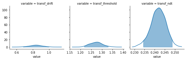
You can simply plot the model’s posteriors using plot_posteriors:

[4]:

model_fit_ddm.plot_posteriors();

../_images/notebooks_inspect_model_7_0.png

By default, 95% HDIs are shown, but you can also choose to have the posteriors without intervals or BCIs, and change the alpha level:

[5]:

model_fit_rl.plot_posteriors(show_intervals='BCI', alpha_intervals=.01);

../_images/notebooks_inspect_model_9_0.png

Trial-level

Depending on the model specification, you can also extract certain trial-level parameters as numpy ordered dictionaries of n_samples X n_trials shape:

[6]:

model_fit_ddm.trial_samples['drift_t'].shape

[6]:

(2000, 400)

[7]:

model_fit_ddm.trial_samples.keys()

[7]:

odict_keys(['drift_t', 'threshold_t', 'ndt_t'])

[8]:

model_fit_lba.trial_samples.keys() # for the LBA

[8]:

odict_keys(['k_t', 'A_t', 'tau_t', 'drift_cor_t', 'drift_inc_t'])

In the case of a RL model fit on choices alone, you can extract the log probability of accuracy=1 for each trial:

[9]:

model_fit_rl.trial_samples.keys()

[9]:

odict_keys(['log_p_t'])

[10]:

model_fit_rl.trial_samples['log_p_t'].shape

[10]:

(2000, 6464)

Posterior predictives

With get_posterior_predictives_df you get posterior predictives as pandas DataFrames of n_posterior_predictives X n_trials shape:

[11]:

pp = model_fit_rl.get_posterior_predictives_df(n_posterior_predictives=1000)
pp

[11]:

variable	accuracy
trial	1	2	3	4	5	6	7	8	9	10	...	6455	6456	6457	6458	6459	6460	6461	6462	6463	6464
sample
1	1	1	1	1	1	1	0	0	1	0	...	0	1	1	1	1	1	1	1	1	1
2	0	1	1	1	1	1	0	1	1	1	...	0	0	1	1	1	1	1	1	1	1
3	1	1	0	0	0	1	1	0	1	1	...	0	1	1	0	0	0	1	1	1	1
4	0	1	0	1	0	1	1	1	1	1	...	0	0	1	1	1	1	1	1	1	1
5	1	1	1	0	1	1	0	0	1	1	...	0	1	1	1	1	1	1	1	1	0
...	...	...	...	...	...	...	...	...	...	...	...	...	...	...	...	...	...	...	...	...	...
996	1	1	0	0	0	1	0	0	1	1	...	1	0	1	1	1	1	1	1	1	1
997	1	0	0	1	1	0	1	0	1	1	...	0	0	1	0	0	0	1	0	0	1
998	0	0	0	1	1	1	1	0	1	1	...	1	1	1	0	1	0	1	1	1	0
999	1	1	0	0	1	1	1	1	1	1	...	0	0	0	1	1	1	1	0	1	1
1000	0	0	1	1	0	1	0	1	1	1	...	0	0	1	1	1	1	1	1	1	1

1000 rows × 6464 columns

For the DDM, you have additional parameters to tweak the DDM simulations, and you get a DataFrame with a hierarchical column index, for RTs and for accuracy:

[12]:

pp = model_fit_ddm.get_posterior_predictives_df(n_posterior_predictives=100, dt=.001)
pp

[12]:

variable	rt										...	accuracy
trial	1	2	3	4	5	6	7	8	9	10	...	391	392	393	394	395	396	397	398	399	400
sample
1	0.383343	0.662343	0.639343	0.748343	0.775343	1.179343	1.619343	0.398343	1.047343	0.329343	...	0.0	1.0	1.0	0.0	1.0	1.0	1.0	0.0	1.0	1.0
2	0.994124	0.333124	0.549124	0.848124	1.027124	0.310124	0.425124	0.601124	0.476124	0.536124	...	1.0	0.0	1.0	1.0	1.0	1.0	1.0	0.0	1.0	0.0
3	1.307052	0.686052	0.457052	0.343052	0.367052	0.612052	0.284052	0.650052	0.381052	0.615052	...	1.0	1.0	1.0	1.0	0.0	1.0	0.0	1.0	0.0	1.0
4	0.642449	0.535449	0.388449	0.470449	0.649449	0.523449	0.338449	0.557449	0.581449	0.606449	...	1.0	1.0	0.0	0.0	0.0	1.0	1.0	1.0	0.0	1.0
5	0.842697	1.535697	0.721697	0.316697	0.708697	1.516697	0.363697	0.751697	0.417697	0.544697	...	0.0	1.0	1.0	1.0	0.0	1.0	1.0	1.0	1.0	1.0
...	...	...	...	...	...	...	...	...	...	...	...	...	...	...	...	...	...	...	...	...	...
96	0.496667	0.334667	0.872667	0.771667	0.389667	0.434667	0.425667	1.027667	0.433667	0.358667	...	1.0	1.0	1.0	1.0	1.0	0.0	1.0	1.0	1.0	1.0
97	0.328090	0.558090	0.444090	0.516090	1.467090	0.736090	1.013090	0.312090	0.405090	0.328090	...	1.0	0.0	1.0	1.0	1.0	1.0	1.0	1.0	0.0	0.0
98	0.424736	0.395736	0.576736	0.411736	0.324736	0.497736	0.520736	0.741736	0.510736	1.300736	...	0.0	1.0	1.0	1.0	1.0	0.0	1.0	1.0	1.0	0.0
99	1.000664	0.364664	0.521664	0.370664	0.387664	0.732664	0.794664	0.369664	0.780664	0.353664	...	1.0	1.0	0.0	1.0	0.0	1.0	1.0	0.0	1.0	0.0
100	0.956275	0.396275	0.968275	0.416275	0.418275	1.048275	1.015275	0.706275	0.383275	0.395275	...	1.0	1.0	1.0	1.0	1.0	0.0	1.0	1.0	1.0	1.0

100 rows × 800 columns

You can also have posterior predictive summaries with get_posterior_predictives_summary.

Only mean accuracy for RL models fit on choices alone, and also mean RTs, skewness and quantiles for lower and upper boundaries for models fitted on RTs as well.

[13]:

model_fit_rl.get_posterior_predictives_summary()

[13]:

	mean_accuracy
sample
1	0.799814
2	0.802754
3	0.803373
4	0.800743
5	0.806312
...	...
496	0.804301
497	0.809561
498	0.807550
499	0.800588
500	0.793472

500 rows × 1 columns

[14]:

model_fit_ddm.get_posterior_predictives_summary()

[14]:

	mean_accuracy	mean_rt	skewness	quant_10_rt_low	quant_30_rt_low	quant_50_rt_low	quant_70_rt_low	quant_90_rt_low	quant_10_rt_up	quant_30_rt_up	quant_50_rt_up	quant_70_rt_up	quant_90_rt_up
sample
1	0.6650	0.670093	2.045784	0.346243	0.460143	0.568843	0.761643	1.152343	0.351843	0.434843	0.550343	0.720843	1.103843
2	0.7500	0.658724	1.576743	0.392724	0.471524	0.565624	0.725624	1.049824	0.348024	0.423524	0.567624	0.703324	1.168924
3	0.7025	0.669302	2.188532	0.363052	0.480652	0.589052	0.779852	1.210852	0.348052	0.455052	0.546052	0.723052	1.068052
4	0.7875	0.640931	2.890019	0.361849	0.446049	0.526449	0.699049	1.110649	0.363849	0.432649	0.543449	0.695449	0.987649
5	0.7625	0.632817	1.456125	0.338897	0.389897	0.481697	0.626897	1.060897	0.361097	0.442697	0.559697	0.754097	1.007497
...	...	...	...	...	...	...	...	...	...	...	...	...	...
496	0.6950	0.615908	1.971778	0.352350	0.408850	0.505750	0.665450	0.982550	0.337250	0.435350	0.543750	0.687050	1.004750
497	0.8025	0.651565	2.103909	0.376220	0.435420	0.567020	0.728620	1.113820	0.352020	0.434020	0.536020	0.710020	1.085020
498	0.7525	0.604910	1.602822	0.328585	0.448785	0.573785	0.717585	0.966385	0.340785	0.429785	0.519785	0.662785	0.956785
499	0.7425	0.624212	1.663869	0.346202	0.433202	0.536402	0.619802	0.957202	0.347602	0.451402	0.552402	0.722202	1.003002
500	0.7625	0.636005	2.907804	0.344582	0.429582	0.522382	0.681182	1.085382	0.350382	0.440582	0.537382	0.698582	1.021982

500 rows × 13 columns

You can also specify which quantiles you are interested in:

[15]:

model_fit_lba.get_posterior_predictives_summary(n_posterior_predictives=200, quantiles=[.1, .5, .9])

[15]:

	mean_accuracy	mean_rt	skewness	quant_10_rt_incorrect	quant_50_rt_incorrect	quant_90_rt_incorrect	quant_10_rt_correct	quant_50_rt_correct	quant_90_rt_correct
sample
1	0.858333	1.721248	1.746695	1.477207	1.835347	2.437212	1.289665	1.589248	2.239182
2	0.850000	1.711749	2.070015	1.353934	1.743663	2.418908	1.249635	1.564929	2.175558
3	0.812500	1.737245	1.874562	1.516550	1.909714	2.711531	1.215915	1.550399	2.272305
4	0.875000	1.629739	1.314279	1.337575	1.594347	2.075680	1.219060	1.536317	2.125802
5	0.841667	1.648190	2.309592	1.304721	1.557302	2.144594	1.228440	1.531487	2.100375
...	...	...	...	...	...	...	...	...	...
196	0.883333	1.719413	2.057477	1.576292	1.939482	2.982563	1.218782	1.544592	2.283167
197	0.908333	1.623029	1.669531	1.286818	1.684597	2.031900	1.211736	1.512554	2.172847
198	0.891667	167.991497	15.491932	1.290854	1.626846	3.500035	1.209622	1.526332	2.445680
199	0.904167	1.672464	4.330050	1.579026	2.011868	2.988423	1.209593	1.535032	1.992702
200	0.891667	1.662455	1.442103	1.374941	1.719873	2.295363	1.249559	1.578828	2.195988

200 rows × 9 columns

Finally, you can get summary for grouping variables (e.g., experimental conditions, trial blocks, etc.) in your data:

[16]:

model_fit_lba.get_grouped_posterior_predictives_summary(n_posterior_predictives=200,
                                                        grouping_vars=['block_label'],
                                                        quantiles=[.3, .5, .7])

[16]:

		mean_accuracy	mean_rt	skewness	quant_30_rt_incorrect	quant_30_rt_correct	quant_50_rt_incorrect	quant_50_rt_correct	quant_70_rt_incorrect	quant_70_rt_correct
block_label	sample
1	1	0.8875	1.742559	0.838222	1.958646	1.402651	2.265617	1.637518	2.414924	1.812356
	2	0.8250	1.667581	2.036401	1.490616	1.386556	1.690442	1.539333	1.996045	1.740201
	3	0.7875	1.727859	1.586878	1.890115	1.314495	2.045244	1.469067	2.167337	1.671310
	4	0.8500	1.683817	6.404095	1.440239	1.336986	1.638169	1.467766	1.874202	1.667109
	5	0.9000	1.625880	2.086927	1.694815	1.334574	1.804016	1.481553	1.877418	1.693119
...	...	...	...	...	...	...	...	...	...	...
3	196	0.9000	1.725673	1.756656	1.776924	1.402891	1.912637	1.556986	1.987094	1.743893
	197	0.8500	1.699036	2.265547	1.630694	1.350169	1.696332	1.519048	2.194706	1.645663
	198	0.9125	1.772827	3.916904	1.515939	1.358824	1.594244	1.478403	2.743708	1.674592
	199	0.8375	1.717850	2.060856	1.609815	1.404633	1.786825	1.567322	1.928092	1.769137
	200	0.8500	1.685803	0.829624	1.469060	1.422103	1.654015	1.567095	1.986281	1.827734

600 rows × 9 columns

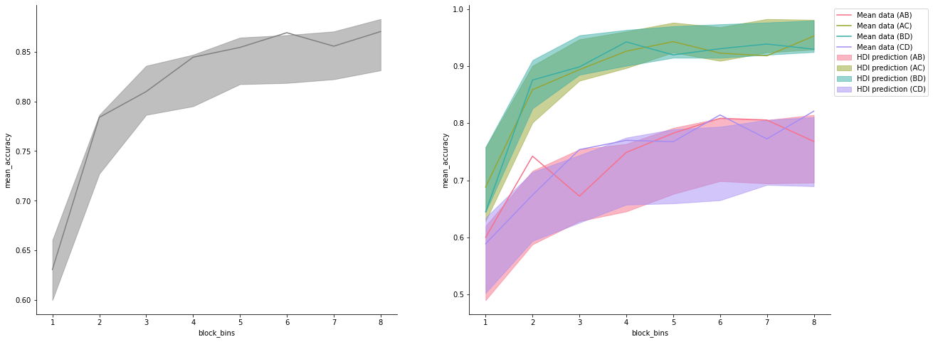
Plot posterior predictives

You can plot posterior predictives similarly, both ungrouped (across all trials) or grouped (across conditions, trial blocks, etc.plot_mean_posterior_predictives).

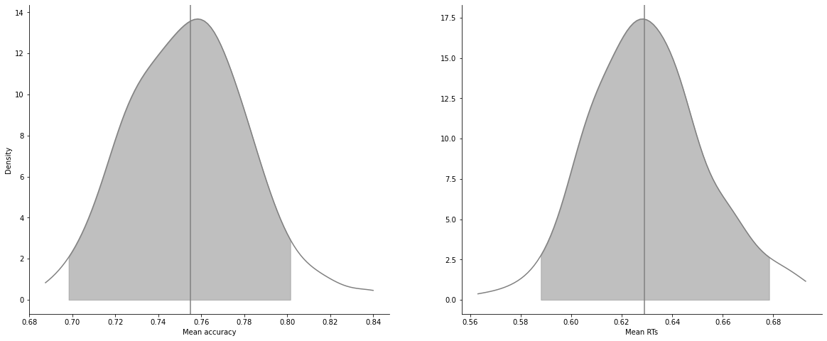
For RT models, you have both mean plots, and quantile plots:

[17]:

model_fit_ddm.plot_mean_posterior_predictives(n_posterior_predictives=200);

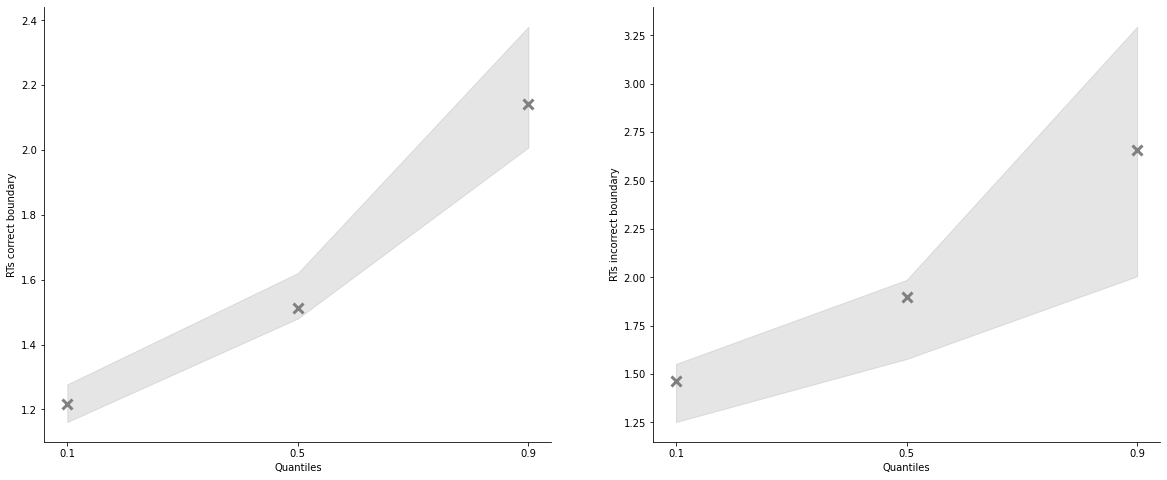
../_images/notebooks_inspect_model_31_0.png

Quantile plots have 2 main visualization options, “shades” and “lines”, and you can specify again which quantiles you want, which in tervals and alpha levels:

[18]:

model_fit_lba.plot_quantiles_posterior_predictives(n_posterior_predictives=200);

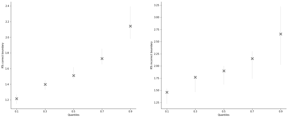
../_images/notebooks_inspect_model_33_0.png

[19]:

model_fit_lba.plot_quantiles_posterior_predictives(n_posterior_predictives=200,
                                                   kind='shades',
                                                   quantiles=[.1, .5, .9]);

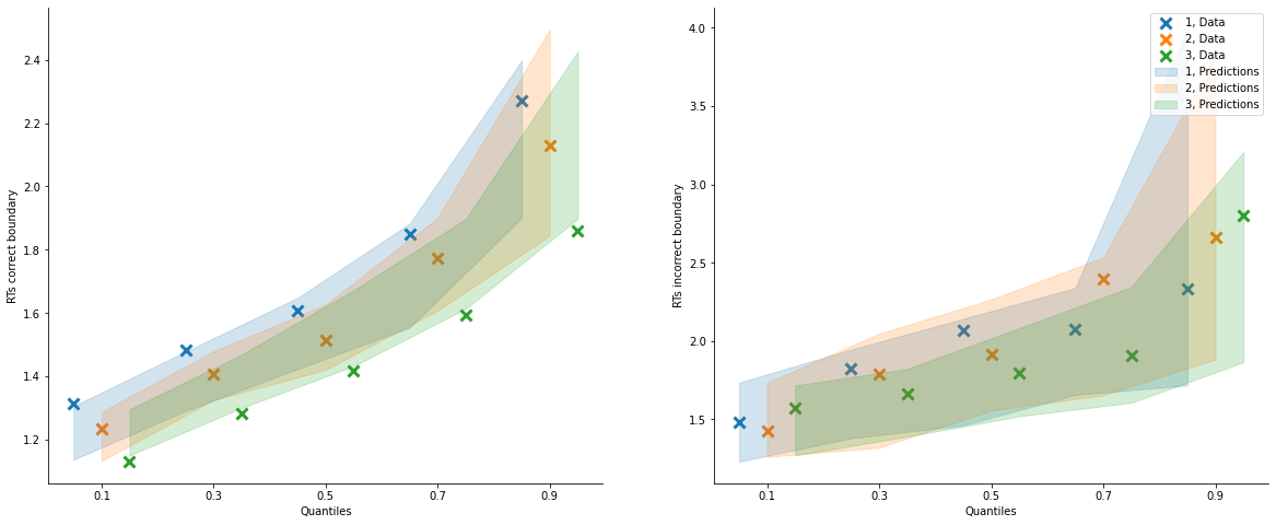
../_images/notebooks_inspect_model_34_0.png

[20]:

model_fit_lba.plot_quantiles_grouped_posterior_predictives(
    n_posterior_predictives=100,
    grouping_var='block_label',
    kind='shades',
    quantiles=[.1, .3, .5, .7, .9]);

../_images/notebooks_inspect_model_35_0.png

[21]:

# Define new grouping variables:

import pandas as pd
import numpy as np

data = model_fit_rl.data_info['data']

# add a column to the data to group trials across learning blocks
data['block_bins'] = pd.cut(data.trial_block, 8, labels=np.arange(1, 9))

# add a column to define which choice pair is shown in that trial
data['choice_pair'] = 'AB'
data.loc[(data.cor_option == 3) & (data.inc_option == 1), 'choice_pair'] = 'AC'
data.loc[(data.cor_option == 4) & (data.inc_option == 2), 'choice_pair'] = 'BD'
data.loc[(data.cor_option == 4) & (data.inc_option == 3), 'choice_pair'] = 'CD'

[22]:

import matplotlib.pyplot as plt
import seaborn as sns

fig, axes = plt.subplots(1, 2, figsize=(20,8))

model_fit_rl.plot_mean_grouped_posterior_predictives(grouping_vars=['block_bins'], n_posterior_predictives=500, ax=axes[0])

model_fit_rl.plot_mean_grouped_posterior_predictives(grouping_vars=['block_bins', 'choice_pair'],
                                                     n_posterior_predictives=500, ax=axes[1])

sns.despine()

../_images/notebooks_inspect_model_37_0.png