Parameter recovery of the DDM with starting point bias
[1]:
import rlssm
import pandas as pd
Simulate individual data
[2]:
from rlssm.random import simulate_ddm
[3]:
data = simulate_ddm(
    n_trials=400,
    gen_drift=.8,
    gen_threshold=1.3,
    gen_ndt=.23,
    gen_rel_sp=.6)
[4]:
data.describe()[['rt', 'accuracy']]
[4]:
| rt | accuracy | |
|---|---|---|
| count | 400.000000 | 400.00000 |
| mean | 0.583140 | 0.81750 |
| std | 0.296395 | 0.38674 |
| min | 0.257000 | 0.00000 |
| 25% | 0.366000 | 1.00000 |
| 50% | 0.493500 | 1.00000 |
| 75% | 0.706500 | 1.00000 |
| max | 1.916000 | 1.00000 |
Initialize the model
[5]:
model = rlssm.DDModel(hierarchical_levels = 1, starting_point_bias=True)
Using cached StanModel
Fit
[6]:
# sampling parameters
n_iter = 3000
n_chains = 2
n_thin = 1

# bayesian model, change default priors:
drift_priors = {'mu':1, 'sd':3}
threshold_priors = {'mu':-1, 'sd':3}
ndt_priors = {'mu':-1, 'sd':1}
[7]:
model_fit = model.fit(
    data,
    drift_priors=drift_priors,
    threshold_priors=threshold_priors,
    ndt_priors=ndt_priors,
    thin = n_thin,
    iter = n_iter,
    chains = n_chains,
    verbose = False)
Fitting the model using the priors:
drift_priors {'mu': 1, 'sd': 3}
threshold_priors {'mu': -1, 'sd': 3}
ndt_priors {'mu': -1, 'sd': 1}
rel_sp_priors {'mu': 0, 'sd': 0.8}
WARNING:pystan:Maximum (flat) parameter count (1000) exceeded: skipping diagnostic tests for n_eff and Rhat.
To run all diagnostics call pystan.check_hmc_diagnostics(fit)
Checks MCMC diagnostics:
n_eff / iter looks reasonable for all parameters
0.0 of 3000 iterations ended with a divergence (0.0%)
0 of 3000 iterations saturated the maximum tree depth of 10 (0.0%)
E-BFMI indicated no pathological behavior
get Rhat
[8]:
model_fit.rhat
[8]:
| rhat | variable | |
|---|---|---|
| 0 | 1.002813 | drift |
| 1 | 1.000353 | threshold |
| 2 | 0.999921 | ndt |
| 3 | 1.003156 | rel_sp |
calculate wAIC
[9]:
model_fit.waic
[9]:
{'lppd': -122.26126045695726,
 'p_waic': 3.682425753566376,
 'waic': 251.88737242104727,
 'waic_se': 47.269086540763105}
Posteriors
[10]:
model_fit.samples.describe()
[10]:
| chain | draw | transf_drift | transf_threshold | transf_ndt | transf_rel_sp | |
|---|---|---|---|---|---|---|
| count | 3000.000000 | 3000.000000 | 3000.000000 | 3000.000000 | 3000.000000 | 3000.000000 |
| mean | 0.500000 | 749.500000 | 0.792928 | 1.306639 | 0.233079 | 0.604580 |
| std | 0.500083 | 433.084792 | 0.103006 | 0.033952 | 0.004736 | 0.019013 |
| min | 0.000000 | 0.000000 | 0.338697 | 1.204520 | 0.214251 | 0.537698 |
| 25% | 0.000000 | 374.750000 | 0.721867 | 1.283811 | 0.230113 | 0.591341 |
| 50% | 0.500000 | 749.500000 | 0.793180 | 1.306182 | 0.233424 | 0.604716 |
| 75% | 1.000000 | 1124.250000 | 0.863523 | 1.329765 | 0.236436 | 0.617648 |
| max | 1.000000 | 1499.000000 | 1.242643 | 1.431171 | 0.247481 | 0.668216 |
[11]:
import seaborn as sns
sns.set(context = "talk",
        style = "white",
        palette = "husl",
        rc={'figure.figsize':(15, 8)})
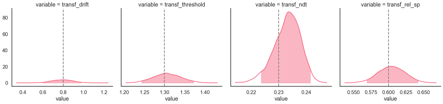
Here we plot the estimated posterior distributions against the generating parameters, to see whether the model parameters are recovering well:
[12]:
g = model_fit.plot_posteriors(height=5, show_intervals='HDI')

for i, ax in enumerate(g.axes.flatten()):
    ax.axvline(data[['drift', 'threshold', 'ndt', 'rel_sp']].mean().values[i], color='grey', linestyle='--')