Fit a RL model on individual data
[1]:
import rlssm
import pandas as pd
import os
Import individual data
[2]:
# import some example data:
data = rlssm.load_example_dataset(hierarchical_levels = 1)

data.head()
[2]:
| participant | block_label | trial_block | f_cor | f_inc | cor_option | inc_option | times_seen | rt | accuracy | |
|---|---|---|---|---|---|---|---|---|---|---|
| 0 | 20 | 1 | 1 | 46 | 46 | 4 | 2 | 1 | 2.574407 | 1 |
| 1 | 20 | 1 | 2 | 60 | 33 | 4 | 2 | 2 | 1.952774 | 1 |
| 2 | 20 | 1 | 3 | 32 | 44 | 2 | 1 | 2 | 2.074999 | 0 |
| 3 | 20 | 1 | 4 | 56 | 40 | 4 | 2 | 3 | 2.320916 | 0 |
| 4 | 20 | 1 | 5 | 34 | 32 | 2 | 1 | 3 | 1.471107 | 1 |
Initialize the model
[3]:
# you can "turn on and off" different mechanisms:
model = rlssm.RLModel_2A(hierarchical_levels = 1,
                         increasing_sensitivity = False,
                         separate_learning_rates = True)
Using cached StanModel
[4]:
model.priors
[4]:
{'sensitivity_priors': {'mu': 1, 'sd': 50},
 'alpha_pos_priors': {'mu': 0, 'sd': 1},
 'alpha_neg_priors': {'mu': 0, 'sd': 1}}
Fit
[5]:
# sampling parameters
n_iter = 2000
n_chains = 2
n_thin = 1

# learning parameters
K = 4 # n options in a learning block (participants see 2 at a time)
initial_value_learning = 27.5 # intitial learning value (Q0)
[6]:
model_fit = model.fit(
    data,
    K,
    initial_value_learning,
    sensitivity_priors={'mu': 0, 'sd': 5},
    thin = n_thin,
    iter = n_iter,
    chains = n_chains,
    verbose = False)
Fitting the model using the priors:
sensitivity_priors {'mu': 0, 'sd': 5}
alpha_pos_priors {'mu': 0, 'sd': 1}
alpha_neg_priors {'mu': 0, 'sd': 1}
WARNING:pystan:n_eff / iter below 0.001 indicates that the effective sample size has likely been overestimated
Checks MCMC diagnostics:
n_eff / iter for parameter log_p_t[1] is 0.0005136779702589292!
E-BFMI below 0.2 indicates you may need to reparameterize your model
n_eff / iter for parameter log_p_t[2] is 0.0005090424204222284!
E-BFMI below 0.2 indicates you may need to reparameterize your model
n_eff / iter for parameter log_p_t[81] is 0.0006137657752379577!
E-BFMI below 0.2 indicates you may need to reparameterize your model
n_eff / iter for parameter log_p_t[161] is 0.000616751650396009!
E-BFMI below 0.2 indicates you may need to reparameterize your model
n_eff / iter for parameter log_lik[1] is 0.0005161261210126754!
E-BFMI below 0.2 indicates you may need to reparameterize your model
n_eff / iter for parameter log_lik[2] is 0.0005103493063252117!
E-BFMI below 0.2 indicates you may need to reparameterize your model
n_eff / iter for parameter log_lik[81] is 0.0009513954236082592!
E-BFMI below 0.2 indicates you may need to reparameterize your model
n_eff / iter below 0.001 indicates that the effective sample size has likely been overestimated
0.0 of 2000 iterations ended with a divergence (0.0%)
0 of 2000 iterations saturated the maximum tree depth of 10 (0.0%)
E-BFMI indicated no pathological behavior
get Rhat
[7]:
model_fit.rhat
[7]:
| rhat | variable | |
|---|---|---|
| 0 | 0.999890 | alpha_pos |
| 1 | 1.000694 | alpha_neg |
| 2 | 1.000057 | sensitivity |
get wAIC
[8]:
model_fit.waic
[8]:
{'lppd': -76.0013341137295,
 'p_waic': 2.584147075766782,
 'waic': 157.17096237899256,
 'waic_se': 15.860333370240344}
Posteriors
[9]:
model_fit.samples.describe()
[9]:
| chain | draw | transf_alpha_pos | transf_alpha_neg | transf_sensitivity | |
|---|---|---|---|---|---|
| count | 2000.000000 | 2000.000000 | 2000.000000 | 2000.000000 | 2000.000000 |
| mean | 0.500000 | 499.500000 | 0.114611 | 0.362081 | 0.345694 |
| std | 0.500125 | 288.747186 | 0.063520 | 0.180011 | 0.057914 |
| min | 0.000000 | 0.000000 | 0.020200 | 0.010799 | 0.187258 |
| 25% | 0.000000 | 249.750000 | 0.070945 | 0.230730 | 0.306195 |
| 50% | 0.500000 | 499.500000 | 0.097523 | 0.329723 | 0.339720 |
| 75% | 1.000000 | 749.250000 | 0.141440 | 0.449876 | 0.376828 |
| max | 1.000000 | 999.000000 | 0.567216 | 0.995145 | 0.789082 |
[10]:
import seaborn as sns
sns.set(context = "talk",
        style = "white",
        palette = "husl",
        rc={'figure.figsize':(15, 8)})
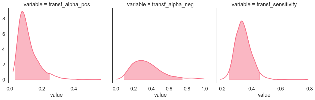
[11]:
model_fit.plot_posteriors(height=5, show_intervals="HDI", alpha_intervals=.05);
Posterior predictives
Ungrouped
[12]:
pp = model_fit.get_posterior_predictives_df(n_posterior_predictives=1000)
pp
[12]:
| variable | accuracy | ||||||||||||||||||||
|---|---|---|---|---|---|---|---|---|---|---|---|---|---|---|---|---|---|---|---|---|---|
| trial | 1 | 2 | 3 | 4 | 5 | 6 | 7 | 8 | 9 | 10 | ... | 231 | 232 | 233 | 234 | 235 | 236 | 237 | 238 | 239 | 240 |
| sample | |||||||||||||||||||||
| 1 | 0 | 1 | 0 | 1 | 1 | 0 | 1 | 1 | 0 | 1 | ... | 1 | 1 | 1 | 1 | 1 | 1 | 1 | 0 | 1 | 1 |
| 2 | 1 | 1 | 0 | 1 | 1 | 1 | 1 | 1 | 1 | 1 | ... | 0 | 1 | 1 | 1 | 1 | 1 | 1 | 0 | 1 | 1 |
| 3 | 1 | 1 | 0 | 1 | 1 | 1 | 1 | 0 | 0 | 1 | ... | 0 | 0 | 1 | 0 | 1 | 0 | 1 | 1 | 0 | 1 |
| 4 | 0 | 0 | 1 | 1 | 0 | 1 | 0 | 1 | 0 | 1 | ... | 0 | 1 | 1 | 1 | 1 | 1 | 1 | 1 | 1 | 1 |
| 5 | 0 | 1 | 1 | 1 | 1 | 1 | 1 | 1 | 0 | 1 | ... | 0 | 0 | 1 | 1 | 1 | 1 | 1 | 1 | 1 | 1 |
| ... | ... | ... | ... | ... | ... | ... | ... | ... | ... | ... | ... | ... | ... | ... | ... | ... | ... | ... | ... | ... | ... |
| 996 | 1 | 1 | 1 | 1 | 1 | 0 | 1 | 0 | 1 | 1 | ... | 1 | 1 | 1 | 1 | 1 | 0 | 0 | 0 | 0 | 1 |
| 997 | 1 | 0 | 1 | 1 | 1 | 0 | 1 | 1 | 0 | 0 | ... | 1 | 1 | 1 | 0 | 1 | 1 | 1 | 1 | 1 | 1 |
| 998 | 0 | 1 | 1 | 1 | 1 | 1 | 0 | 0 | 0 | 1 | ... | 0 | 0 | 1 | 1 | 1 | 0 | 1 | 1 | 1 | 1 |
| 999 | 1 | 1 | 1 | 1 | 1 | 1 | 1 | 0 | 0 | 0 | ... | 1 | 0 | 1 | 1 | 1 | 0 | 1 | 1 | 0 | 1 |
| 1000 | 0 | 0 | 1 | 0 | 1 | 1 | 1 | 1 | 0 | 1 | ... | 0 | 1 | 1 | 1 | 1 | 0 | 1 | 1 | 1 | 1 |
1000 rows × 240 columns
[13]:
pp_summary = model_fit.get_posterior_predictives_summary(n_posterior_predictives=1000)
pp_summary
[13]:
| mean_accuracy | |
|---|---|
| sample | |
| 1 | 0.804167 |
| 2 | 0.804167 |
| 3 | 0.800000 |
| 4 | 0.883333 |
| 5 | 0.825000 |
| ... | ... |
| 996 | 0.833333 |
| 997 | 0.908333 |
| 998 | 0.887500 |
| 999 | 0.845833 |
| 1000 | 0.900000 |
1000 rows × 1 columns
[14]:
import matplotlib.pyplot as plt
fig, ax = plt.subplots(1, 1, figsize=(5, 5))

model_fit.plot_mean_posterior_predictives(n_posterior_predictives=500, ax=ax, show_intervals='HDI')

ax.set_ylabel('Density')
ax.set_xlabel('Mean accuracy')

sns.despine()

Grouped
[15]:
import numpy as np
[16]:
# Define new grouping variables, in this case, for the different choice pairs, but any grouping var can do
data['choice_pair'] = 'AB'
data.loc[(data.cor_option == 3) & (data.inc_option == 1), 'choice_pair'] = 'AC'
data.loc[(data.cor_option == 4) & (data.inc_option == 2), 'choice_pair'] = 'BD'
data.loc[(data.cor_option == 4) & (data.inc_option == 3), 'choice_pair'] = 'CD'

data['block_bins'] = pd.cut(data.trial_block, 8, labels=np.arange(1, 9))
[17]:
model_fit.get_grouped_posterior_predictives_summary(grouping_vars=['block_label', 'block_bins', 'choice_pair'],
                                                    n_posterior_predictives=500)
[17]:
| mean_accuracy | ||||
|---|---|---|---|---|
| block_label | block_bins | choice_pair | sample | |
| 1 | 1 | AB | 1 | 0.800000 |
| 2 | 0.200000 | |||
| 3 | 0.600000 | |||
| 4 | 0.800000 | |||
| 5 | 0.800000 | |||
| ... | ... | ... | ... | ... |
| 3 | 8 | CD | 496 | 1.000000 |
| 497 | 0.666667 | |||
| 498 | 0.333333 | |||
| 499 | 0.333333 | |||
| 500 | 0.333333 |
46000 rows × 1 columns
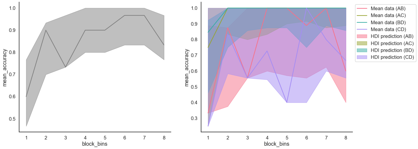
[18]:
import matplotlib.pyplot as plt

fig, axes = plt.subplots(1, 2, figsize=(20,8))

model_fit.plot_mean_grouped_posterior_predictives(grouping_vars=['block_bins'], n_posterior_predictives=500, ax=axes[0])

model_fit.plot_mean_grouped_posterior_predictives(grouping_vars=['block_bins', 'choice_pair'], n_posterior_predictives=500, ax=axes[1])

sns.despine()