Fit the LBA on individual data

[1]:

import rlssm
import pandas as pd
import os

Import individual data

[2]:

# import some example data:
data = rlssm.load_example_dataset(hierarchical_levels = 1)

data.head()

[2]:

	participant	block_label	trial_block	f_cor	f_inc	cor_option	inc_option	times_seen	rt	accuracy
0	20	1	1	46	46	4	2	1	2.574407	1
1	20	1	2	60	33	4	2	2	1.952774	1
2	20	1	3	32	44	2	1	2	2.074999	0
3	20	1	4	56	40	4	2	3	2.320916	0
4	20	1	5	34	32	2	1	3	1.471107	1

Initialize the model

[3]:

model = rlssm.LBAModel_2A(hierarchical_levels = 1)

Using cached StanModel

Fit

[4]:

# sampling parameters
n_iter = 1000
n_chains = 2
n_thin = 5

[5]:

model_fit = model.fit(
    data,
    thin = n_thin,
    iter = n_iter,
    chains = n_chains)

Fitting the model using the priors:
drift_priors {'mu': 1, 'sd': 5}
k_priors {'mu': 1, 'sd': 1}
A_priors {'mu': 0.3, 'sd': 1}
tau_priors {'mu': 0, 'sd': 1}

WARNING:pystan:Maximum (flat) parameter count (1000) exceeded: skipping diagnostic tests for n_eff and Rhat.
To run all diagnostics call pystan.check_hmc_diagnostics(fit)

Checks MCMC diagnostics:
n_eff / iter looks reasonable for all parameters
0.0 of 200 iterations ended with a divergence (0.0%)
0 of 200 iterations saturated the maximum tree depth of 10 (0.0%)
E-BFMI indicated no pathological behavior

Get rhat

[6]:

model_fit.rhat

[6]:

	rhat	variable
0	0.996595	k
1	0.996693	A
2	0.995655	tau
3	0.999796	drift_cor
4	1.002850	drift_inc

Get WAIC

[7]:

model_fit.waic

[7]:

{'lppd': -195.9117676732156,
 'p_waic': 3.4080101153548954,
 'waic': 398.639555577141,
 'waic_se': 35.24758887155065}

Save results

[8]:

model_fit.to_pickle()

Saving file as: /Users/laurafontanesi/git/rlssm/docs/notebooks/LBA_2A.pkl

Posteriors

[9]:

model_fit.samples.describe()

[9]:

	chain	draw	transf_k	transf_A	transf_tau	transf_drift_cor	transf_drift_inc
count	200.000000	200.000000	200.000000	200.000000	200.000000	200.000000	200.000000
mean	0.500000	49.500000	3.072969	1.282488	0.420315	3.123329	1.517988
std	0.501255	28.938507	0.617627	0.545432	0.097345	0.264801	0.256313
min	0.000000	0.000000	1.547620	0.199475	0.193221	2.546426	0.849490
25%	0.000000	24.750000	2.617696	0.853162	0.356208	2.950180	1.360080
50%	0.500000	49.500000	3.097387	1.279160	0.425263	3.109816	1.517640
75%	1.000000	74.250000	3.441474	1.622801	0.477226	3.265753	1.679263
max	1.000000	99.000000	4.636813	2.929345	0.698922	3.853958	2.140647

[10]:

import seaborn as sns
sns.set(context = "talk",
        style = "white",
        palette = "husl",
        rc={'figure.figsize':(15, 8)})

[11]:

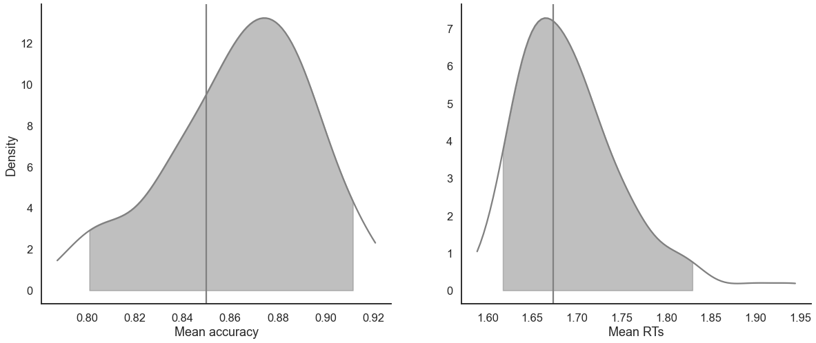
model_fit.plot_posteriors(height=5, show_intervals='HDI');

../_images/notebooks_LBA_2A_fitting_18_0.png

Posterior predictives

Ungrouped

[12]:

pp = model_fit.get_posterior_predictives_df(n_posterior_predictives=100)
pp

[12]:

variable	rt										...	accuracy
trial	1	2	3	4	5	6	7	8	9	10	...	231	232	233	234	235	236	237	238	239	240
sample
1	2.246846	1.537963	1.249976	2.667635	1.394088	1.185661	1.775463	1.299116	2.344744	1.585738	...	1.0	1.0	1.0	1.0	0.0	1.0	1.0	1.0	1.0	1.0
2	1.474279	1.317326	1.281292	1.776970	1.338612	1.595272	1.423343	1.411392	1.368143	1.718686	...	1.0	0.0	1.0	1.0	0.0	0.0	1.0	1.0	1.0	1.0
3	1.769881	1.248670	2.000013	2.477428	1.417273	1.537488	1.298886	2.047417	1.673906	1.490852	...	1.0	1.0	1.0	1.0	0.0	1.0	1.0	1.0	1.0	1.0
4	1.218720	1.806578	1.491374	1.556123	1.754127	2.173220	1.786404	1.423031	1.509262	1.651425	...	1.0	1.0	1.0	1.0	1.0	1.0	1.0	1.0	1.0	1.0
5	1.505410	1.545240	1.263004	1.981529	1.742220	1.447841	2.140920	1.298421	1.297520	1.534183	...	1.0	1.0	1.0	0.0	0.0	1.0	1.0	1.0	1.0	1.0
...	...	...	...	...	...	...	...	...	...	...	...	...	...	...	...	...	...	...	...	...	...
96	2.114076	1.682352	1.292053	1.290883	1.631570	2.536921	1.475092	1.839493	1.549875	1.748721	...	1.0	1.0	1.0	1.0	1.0	1.0	1.0	1.0	1.0	1.0
97	1.515118	1.732291	7.900185	1.992388	1.701881	1.195694	1.765124	2.120031	1.681817	1.935664	...	1.0	0.0	1.0	1.0	1.0	1.0	1.0	1.0	1.0	1.0
98	1.934512	1.704758	3.664648	2.025907	2.636455	1.388794	1.289439	1.364305	1.641123	1.961389	...	1.0	1.0	1.0	1.0	1.0	1.0	1.0	1.0	1.0	0.0
99	1.485397	1.458125	1.561393	1.374246	1.817840	1.899995	2.221972	2.021029	1.958976	1.611125	...	1.0	1.0	1.0	1.0	1.0	1.0	1.0	0.0	1.0	0.0
100	1.858069	1.869365	1.464518	1.568417	2.022131	1.332558	1.296797	2.512003	1.955222	3.026658	...	0.0	1.0	1.0	1.0	1.0	1.0	1.0	1.0	1.0	0.0

100 rows × 480 columns

[13]:

pp_summary = model_fit.get_posterior_predictives_summary(n_posterior_predictives=100)
pp_summary

[13]:

	mean_accuracy	mean_rt	skewness	quant_10_rt_incorrect	quant_30_rt_incorrect	quant_50_rt_incorrect	quant_70_rt_incorrect	quant_90_rt_incorrect	quant_10_rt_correct	quant_30_rt_correct	quant_50_rt_correct	quant_70_rt_correct	quant_90_rt_correct
sample
1	0.854167	1.664804	2.165810	1.506785	1.669890	1.752361	2.038205	2.385568	1.221533	1.359931	1.511616	1.739581	2.151703
2	0.862500	1.682668	3.158625	1.368550	1.540713	1.674629	2.156115	2.884746	1.240682	1.375500	1.534844	1.744025	2.127136
3	0.850000	1.712393	1.725298	1.613360	1.732978	1.990309	2.124092	2.672556	1.243860	1.403816	1.528488	1.743321	2.166606
4	0.887500	1.619813	2.537257	1.331044	1.556282	1.776372	2.082097	2.355689	1.149061	1.302143	1.471107	1.648440	2.088338
5	0.845833	1.768796	2.713919	1.382418	1.583290	1.743878	2.181400	2.802916	1.258256	1.455523	1.567858	1.793322	2.336169
...	...	...	...	...	...	...	...	...	...	...	...	...	...
96	0.858333	1.679296	2.592582	1.538260	1.704401	1.905312	2.145374	2.677621	1.191991	1.364760	1.517171	1.705111	2.255572
97	0.887500	1.705270	8.036846	1.314066	1.598821	1.771878	2.127968	2.772499	1.191808	1.345362	1.502895	1.700021	2.239710
98	0.891667	1.674279	2.983261	1.416547	1.601738	1.762865	1.999681	2.596806	1.222192	1.372858	1.562998	1.767055	2.190829
99	0.812500	1.740113	3.226386	1.337939	1.570886	1.752819	2.034753	2.808015	1.211335	1.442884	1.596091	1.788202	2.252709
100	0.904167	1.803922	4.509639	1.383537	1.553577	1.736791	1.890371	2.585798	1.243580	1.441850	1.608690	1.858538	2.475641

100 rows × 13 columns

[14]:

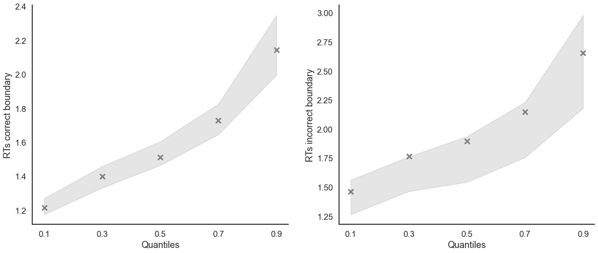
model_fit.plot_mean_posterior_predictives(n_posterior_predictives=100, figsize=(20,8), show_intervals='HDI');

../_images/notebooks_LBA_2A_fitting_23_0.png

[15]:

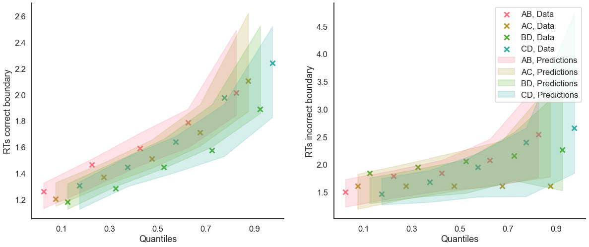
model_fit.plot_quantiles_posterior_predictives(n_posterior_predictives=100, kind='shades');

../_images/notebooks_LBA_2A_fitting_24_0.png

Grouped

[16]:

import numpy as np

[17]:

# Define new grouping variables, in this case, for the different choice pairs, but any grouping var can do
data['choice_pair'] = 'AB'
data.loc[(data.cor_option == 3) & (data.inc_option == 1), 'choice_pair'] = 'AC'
data.loc[(data.cor_option == 4) & (data.inc_option == 2), 'choice_pair'] = 'BD'
data.loc[(data.cor_option == 4) & (data.inc_option == 3), 'choice_pair'] = 'CD'

data['block_bins'] = pd.cut(data.trial_block, 8, labels=np.arange(1, 9))

[18]:

model_fit.get_grouped_posterior_predictives_summary(
                grouping_vars=['block_label', 'choice_pair'],
                quantiles=[.3, .5, .7],
                n_posterior_predictives=100)

[18]:

			mean_accuracy	mean_rt	skewness	quant_30_rt_incorrect	quant_30_rt_correct	quant_50_rt_incorrect	quant_50_rt_correct	quant_70_rt_incorrect	quant_70_rt_correct
block_label	choice_pair	sample
1	AB	1	0.85	1.760965	2.793220	2.273896	1.349401	2.481967	1.600919	3.183433	1.703819
		2	0.75	1.791783	1.563911	1.768126	1.315160	2.557145	1.426042	2.614723	1.619165
		3	0.90	1.743365	2.371058	2.337256	1.448736	2.416226	1.615792	2.495196	1.723226
		4	0.85	1.801372	2.994665	1.981311	1.463829	2.114486	1.677760	2.126189	1.782304
		5	0.90	1.617718	3.355427	2.051592	1.385195	2.619649	1.455759	3.187705	1.580824
...	...	...	...	...	...	...	...	...	...	...	...
3	CD	96	0.85	1.659586	-0.079339	1.661425	1.501355	1.726938	1.584971	1.852454	1.809642
		97	0.85	1.524945	1.819670	1.528637	1.322557	1.713642	1.434720	1.860052	1.482929
		98	0.90	1.668617	1.254209	1.800101	1.443070	1.805070	1.491801	1.810039	1.667956
		99	0.75	1.462542	0.138408	1.512019	1.255587	1.536708	1.457608	1.646303	1.573202
		100	0.70	1.609434	0.946274	1.566879	1.516307	1.694011	1.562540	1.858372	1.618214

1200 rows × 9 columns

[19]:

model_fit.get_grouped_posterior_predictives_summary(
                grouping_vars=['block_bins'],
                quantiles=[.3, .5, .7],
                n_posterior_predictives=100)

[19]:

		mean_accuracy	mean_rt	skewness	quant_30_rt_incorrect	quant_30_rt_correct	quant_50_rt_incorrect	quant_50_rt_correct	quant_70_rt_incorrect	quant_70_rt_correct
block_bins	sample
1	1	0.866667	1.725833	1.289234	1.584221	1.460545	1.660907	1.644744	1.729153	1.791533
	2	0.900000	1.752329	1.527601	2.231171	1.498770	2.560241	1.612940	2.708332	1.745022
	3	0.900000	1.686033	0.924488	1.746004	1.332471	1.842445	1.544803	1.884541	1.863387
	4	0.900000	1.732809	1.865226	2.113744	1.246336	2.483196	1.450803	2.575727	1.597772
	5	0.800000	1.635091	2.085413	1.567397	1.324384	1.675482	1.518778	1.730329	1.790997
...	...	...	...	...	...	...	...	...	...	...
8	96	0.966667	1.735385	4.445814	2.664596	1.356872	2.664596	1.475787	2.664596	1.649329
	97	0.833333	1.693073	0.534953	1.727258	1.334572	1.769807	1.583482	1.853036	1.902496
	98	0.866667	1.791996	0.811008	1.669274	1.466517	1.782816	1.642452	1.919534	1.949012
	99	0.900000	1.738719	1.967172	1.483509	1.408075	1.496928	1.619821	2.271276	1.783024
	100	0.866667	1.796386	1.052592	1.761800	1.419787	1.807006	1.594746	1.927432	2.010042

800 rows × 9 columns

[20]:

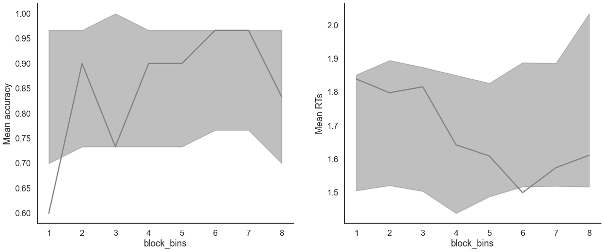
model_fit.plot_mean_grouped_posterior_predictives(grouping_vars=['block_bins'],
                                                  n_posterior_predictives=100,
                                                  figsize=(20,8));

../_images/notebooks_LBA_2A_fitting_30_0.png

[21]:

model_fit.plot_quantiles_grouped_posterior_predictives(
    n_posterior_predictives=100,
    grouping_var='choice_pair',
    kind='shades',
    quantiles=[.1, .3, .5, .7, .9]);

../_images/notebooks_LBA_2A_fitting_31_0.png