Fit the RLDDM on individual data

[1]:

import rlssm
import pandas as pd
import os

Import the data

[2]:

# import some example data:
data = rlssm.load_example_dataset(hierarchical_levels = 1)

data.head()

[2]:

	participant	block_label	trial_block	f_cor	f_inc	cor_option	inc_option	times_seen	rt	accuracy
0	10	1	1	61	52	4	3	1	1.285418	0
1	10	1	2	54	37	4	2	1	1.577622	0
2	10	1	3	51	51	4	3	2	1.564731	0
3	10	1	4	50	35	3	1	2	1.217245	1
4	10	1	5	59	50	4	2	3	1.929781	0

Initialize the model

[3]:

# you can "turn on and off" different mechanisms:
model = rlssm.RLDDModel(hierarchical_levels=1,
                        separate_learning_rates=False,
                        threshold_modulation=False,
                        nonlinear_mapping=True)

Using cached StanModel

Fit

[4]:

# sampling parameters
n_iter = 3000
n_warmup = 1000
n_chains = 2

# learning parameters
K = 4 # n options in a learning block (participants see 2 at a time)
initial_value_learning = 27.5 # intitial learning value (Q0)

[5]:

model_fit = model.fit(
    data,
    K,
    initial_value_learning,
    warmup = n_warmup,
    iter = n_iter,
    chains = n_chains)

Fitting the model using the priors:
alpha_priors {'mu': 0, 'sd': 1}
drift_scaling_priors {'mu': 1, 'sd': 50}
drift_asymptote_priors {'mu': 1, 'sd': 50}
threshold_priors {'mu': 1, 'sd': 5}
ndt_priors {'mu': 1, 'sd': 1}

WARNING:pystan:Maximum (flat) parameter count (1000) exceeded: skipping diagnostic tests for n_eff and Rhat.
To run all diagnostics call pystan.check_hmc_diagnostics(fit)
WARNING:pystan:6 of 4000 iterations ended with a divergence (0.15 %).
WARNING:pystan:Try running with adapt_delta larger than 0.8 to remove the divergences.
WARNING:pystan:6 of 4000 iterations saturated the maximum tree depth of 10 (0.15 %)
WARNING:pystan:Run again with max_treedepth larger than 10 to avoid saturation

Checks MCMC diagnostics:
n_eff / iter looks reasonable for all parameters
6.0 of 4000 iterations ended with a divergence (0.15%)
  Try running with larger adapt_delta to remove the divergences
6 of 4000 iterations saturated the maximum tree depth of 10 (0.15%)
Run again with max_depth set to a larger value to avoid saturation
E-BFMI indicated no pathological behavior

get Rhat

[6]:

model_fit.rhat

[6]:

	rhat	variable
0	1.018417	alpha
1	1.037281	drift_scaling
2	1.027634	drift_asymptote
3	1.000449	threshold
4	1.001236	ndt

get wAIC

[7]:

model_fit.waic

[7]:

{'lppd': -222.10485280567747,
 'p_waic': 4.70099816274729,
 'waic': 453.6117019368495,
 'waic_se': 28.500117385818506}

Posteriors

[8]:

model_fit.samples.describe()

[8]:

	chain	draw	transf_alpha	transf_drift_scaling	transf_drift_asymptote	transf_threshold	transf_ndt
count	4000.000000	4000.000000	4000.000000	4000.000000	4000.000000	4000.000000	4000.000000
mean	0.500000	999.500000	0.037983	0.794183	36.160095	1.873717	0.797365
std	0.500063	577.422379	0.039915	4.429973	30.778307	0.063024	0.010966
min	0.000000	0.000000	0.000057	0.002300	2.043295	1.685766	0.739923
25%	0.000000	499.750000	0.014890	0.013506	9.554932	1.828763	0.790487
50%	0.500000	999.500000	0.027752	0.029816	28.618335	1.873455	0.798071
75%	1.000000	1499.250000	0.048028	0.103515	54.034849	1.915392	0.805142
max	1.000000	1999.000000	0.587557	64.531895	190.530448	2.084672	0.826664

[9]:

import seaborn as sns
sns.set(context = "talk",
        style = "white",
        palette = "husl",
        rc={'figure.figsize':(15, 8)})

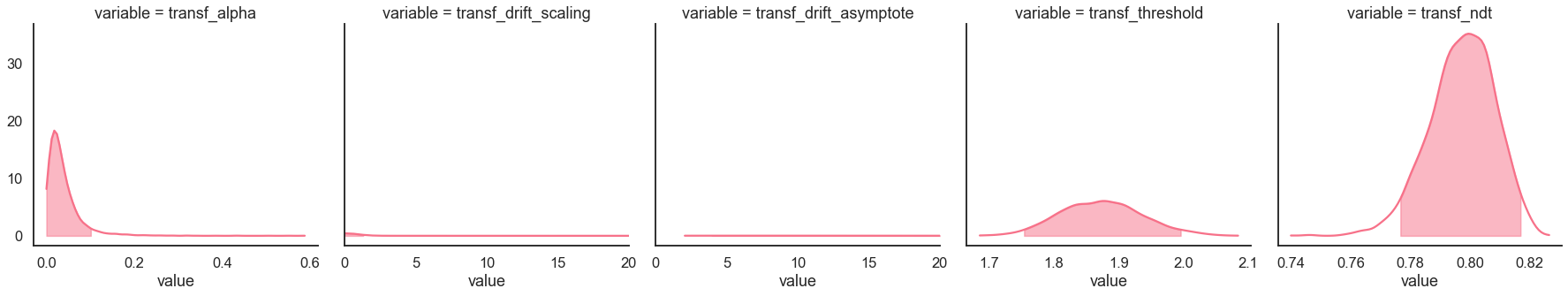
[10]:

g = model_fit.plot_posteriors(height=5, show_intervals='HDI');

g.axes.flat[1].set_xlim(0, 20)
g.axes.flat[2].set_xlim(0, 20);

../_images/notebooks_RLDDM_fitting_16_0.png

Posterior predictives

Ungrouped

[11]:

pp = model_fit.get_posterior_predictives_df(n_posterior_predictives=100)
pp

[11]:

variable	rt										...	accuracy
trial	1	2	3	4	5	6	7	8	9	10	...	230	231	232	233	234	235	236	237	238	239
sample
1	1.262933	1.069933	1.784933	1.543933	1.083933	1.111933	2.414933	1.016933	1.438933	1.144933	...	1.0	0.0	1.0	1.0	1.0	1.0	1.0	1.0	1.0	0.0
2	1.025510	5.076510	1.705510	1.124510	1.230510	1.659510	1.058510	2.201510	1.932510	1.383510	...	1.0	1.0	1.0	1.0	1.0	0.0	1.0	1.0	1.0	0.0
3	1.563506	1.586506	1.463506	1.030506	0.960506	1.705506	1.394506	1.566506	1.668506	1.237506	...	1.0	1.0	0.0	1.0	1.0	1.0	1.0	1.0	0.0	1.0
4	1.377698	1.081698	2.731698	2.004698	1.227698	1.097698	2.421698	2.383698	1.264698	2.216698	...	1.0	1.0	1.0	1.0	1.0	1.0	1.0	1.0	1.0	1.0
5	1.211327	0.994327	1.420327	1.985327	0.982327	1.153327	1.323327	1.587327	1.402327	1.462327	...	1.0	1.0	1.0	1.0	1.0	1.0	1.0	1.0	1.0	1.0
...	...	...	...	...	...	...	...	...	...	...	...	...	...	...	...	...	...	...	...	...	...
96	1.638157	0.958157	1.110157	1.300157	1.791157	1.347157	1.563157	1.162157	1.243157	2.055157	...	1.0	1.0	1.0	1.0	1.0	0.0	1.0	1.0	1.0	1.0
97	1.278817	1.766817	1.079817	1.173817	1.616817	2.170817	1.960817	1.078817	1.794817	1.288817	...	1.0	1.0	1.0	1.0	1.0	1.0	1.0	1.0	1.0	1.0
98	1.075953	1.300953	1.090953	1.380953	1.067953	2.644953	1.694953	1.517953	1.402953	1.505953	...	1.0	1.0	1.0	1.0	1.0	1.0	1.0	1.0	1.0	1.0
99	1.154160	1.308160	1.598160	3.026160	2.950160	0.944160	1.161160	1.392160	1.694160	1.407160	...	1.0	1.0	1.0	1.0	1.0	0.0	1.0	1.0	1.0	1.0
100	2.028603	1.326603	1.547603	1.012603	1.077603	3.032603	1.243603	1.232603	1.043603	0.913603	...	1.0	1.0	1.0	1.0	1.0	0.0	1.0	1.0	1.0	0.0

100 rows × 478 columns

[12]:

pp_summary = model_fit.get_posterior_predictives_summary(n_posterior_predictives=100)
pp_summary

[12]:

	mean_accuracy	mean_rt	skewness	quant_10_rt_low	quant_30_rt_low	quant_50_rt_low	quant_70_rt_low	quant_90_rt_low	quant_10_rt_up	quant_30_rt_up	quant_50_rt_up	quant_70_rt_up	quant_90_rt_up
sample
1	0.736402	1.597975	2.020770	1.046733	1.180133	1.408933	1.834733	2.707733	1.018933	1.226433	1.405433	1.629933	2.320933
2	0.803347	1.568459	2.537627	1.036110	1.224110	1.456510	1.908310	2.555710	1.007610	1.186710	1.328510	1.644910	2.335410
3	0.744770	1.592808	2.887339	1.006506	1.161506	1.417506	1.887506	2.220506	1.027106	1.195906	1.334506	1.637906	2.401806
4	0.748954	1.596832	1.956484	1.062198	1.234398	1.577698	1.925998	2.465298	1.015098	1.157698	1.359698	1.651698	2.269698
5	0.765690	1.517963	2.230927	1.002327	1.154827	1.437327	1.729827	2.573327	1.000527	1.139527	1.300327	1.564927	2.151527
...	...	...	...	...	...	...	...	...	...	...	...	...	...
96	0.686192	1.420931	1.572826	0.967357	1.108957	1.323157	1.570757	2.142957	0.958757	1.081057	1.277157	1.438257	2.128157
97	0.778243	1.513348	3.399520	1.023017	1.141617	1.316817	1.542817	1.993417	1.025817	1.198817	1.376317	1.621317	2.195317
98	0.757322	1.657665	2.967858	1.047453	1.262653	1.514953	1.938653	2.723953	1.015953	1.177953	1.370953	1.686953	2.368953
99	0.761506	1.491198	2.239910	1.002160	1.203360	1.428160	1.722160	2.474160	1.015160	1.135160	1.244660	1.503260	2.128160
100	0.769874	1.476908	2.132750	1.057803	1.188803	1.390603	1.567003	2.074803	0.990203	1.108203	1.276603	1.540803	2.212203

100 rows × 13 columns

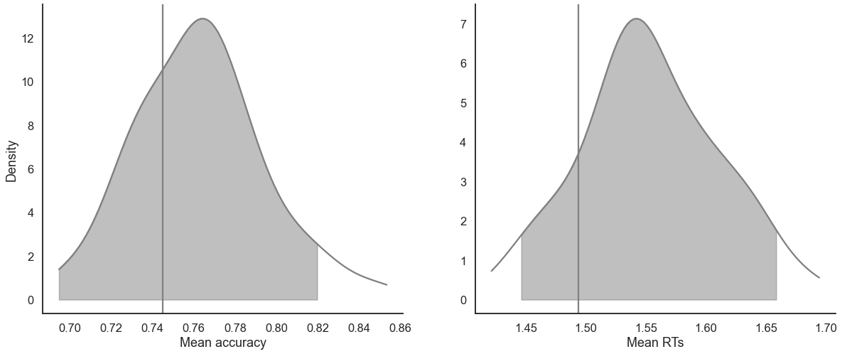
[13]:

model_fit.plot_mean_posterior_predictives(n_posterior_predictives=100, figsize=(20,8), show_intervals='HDI');

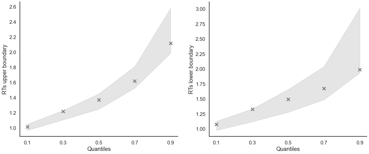
../_images/notebooks_RLDDM_fitting_21_0.png

[14]:

model_fit.plot_quantiles_posterior_predictives(n_posterior_predictives=100, kind='shades');

../_images/notebooks_RLDDM_fitting_22_0.png

Grouped

[15]:

import numpy as np

[16]:

# Define new grouping variables, in this case, for the different choice pairs, but any grouping var can do
data['choice_pair'] = 'AB'
data.loc[(data.cor_option == 3) & (data.inc_option == 1), 'choice_pair'] = 'AC'
data.loc[(data.cor_option == 4) & (data.inc_option == 2), 'choice_pair'] = 'BD'
data.loc[(data.cor_option == 4) & (data.inc_option == 3), 'choice_pair'] = 'CD'

data['block_bins'] = pd.cut(data.trial_block, 8, labels=np.arange(1, 9))

[17]:

model_fit.get_grouped_posterior_predictives_summary(
                grouping_vars=['block_label', 'choice_pair'],
                quantiles=[.3, .5, .7],
                n_posterior_predictives=100)

[17]:

			mean_accuracy	mean_rt	skewness	quant_30_rt_low	quant_30_rt_up	quant_50_rt_low	quant_50_rt_up	quant_70_rt_low	quant_70_rt_up
block_label	choice_pair	sample
1	AB	1	0.75	2.049033	1.861715	1.215533	1.493133	1.261933	1.537933	1.385933	2.341733
		2	0.65	1.672710	1.528835	1.153710	1.194110	1.548510	1.394510	1.751310	1.922710
		3	0.55	1.501656	0.745925	1.239906	1.102506	1.471506	1.159506	1.657906	1.648506
		4	0.75	1.343298	1.370879	1.110298	1.043498	1.464698	1.161698	1.526298	1.313698
		5	0.65	1.492577	2.332409	1.176527	1.166127	1.297327	1.237327	1.693927	1.416327
...	...	...	...	...	...	...	...	...	...	...	...
3	CD	96	0.55	1.266957	1.404526	1.086357	1.191157	1.123157	1.262157	1.181957	1.365157
		97	0.60	1.652267	0.660315	1.150917	1.331017	1.527317	1.603817	2.327617	1.847717
		98	0.55	1.756253	0.798266	1.631753	1.265953	1.652953	1.288953	2.349353	1.884953
		99	0.70	1.721210	3.783809	1.402160	1.234060	1.556660	1.314660	1.684660	1.701360
		100	0.70	1.791353	2.759446	0.991603	1.474003	1.134103	1.665103	1.659103	1.834503

1200 rows × 9 columns

[18]:

model_fit.get_grouped_posterior_predictives_summary(
                grouping_vars=['block_bins'],
                quantiles=[.3, .5, .7],
                n_posterior_predictives=100)

[18]:

		mean_accuracy	mean_rt	skewness	quant_30_rt_low	quant_30_rt_up	quant_50_rt_low	quant_50_rt_up	quant_70_rt_low	quant_70_rt_up
block_bins	sample
1	1	0.700000	1.602333	1.979790	1.158733	1.141933	1.284933	1.326933	1.535933	1.756933
	2	0.566667	1.757410	1.151978	1.383910	1.077710	1.912510	1.238510	2.361110	1.508510
	3	0.466667	1.813140	1.656559	1.101506	1.148406	1.655006	1.530006	1.874006	2.292106
	4	0.566667	1.899765	0.471722	1.463898	1.342298	1.783698	1.718698	2.064898	2.397498
	5	0.433333	1.572861	1.098442	1.180327	1.087927	1.458327	1.264327	1.775127	1.447327
...	...	...	...	...	...	...	...	...	...	...
8	96	0.862069	1.374777	2.498250	1.055157	1.124157	1.142157	1.198157	1.422057	1.367757
	97	0.862069	1.655334	0.906741	1.427517	1.215217	1.499317	1.459817	1.592817	1.846817
	98	0.827586	1.357953	2.034553	1.469153	1.014053	1.689953	1.115453	1.845153	1.261953
	99	0.862069	1.354539	0.819861	1.521060	1.143760	1.748660	1.229160	1.941960	1.382560
	100	0.965517	1.464017	2.051352	1.133603	1.094103	1.133603	1.317603	1.133603	1.514103

800 rows × 9 columns

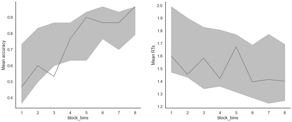
[19]:

model_fit.plot_mean_grouped_posterior_predictives(grouping_vars=['block_bins'],
                                                  n_posterior_predictives=100,
                                                  figsize=(20,8));

../_images/notebooks_RLDDM_fitting_28_0.png

[20]:

model_fit.plot_quantiles_grouped_posterior_predictives(n_posterior_predictives=100,
                                                        grouping_var='choice_pair',
                                                        kind='shades',
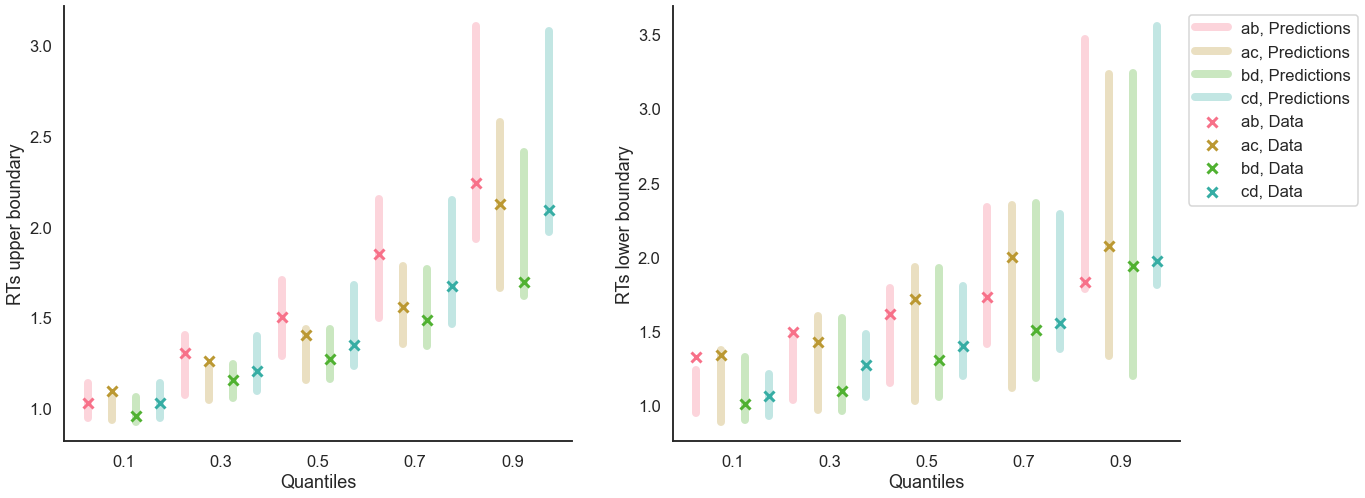
                                                        quantiles=[.1, .3, .5, .7, .9]);

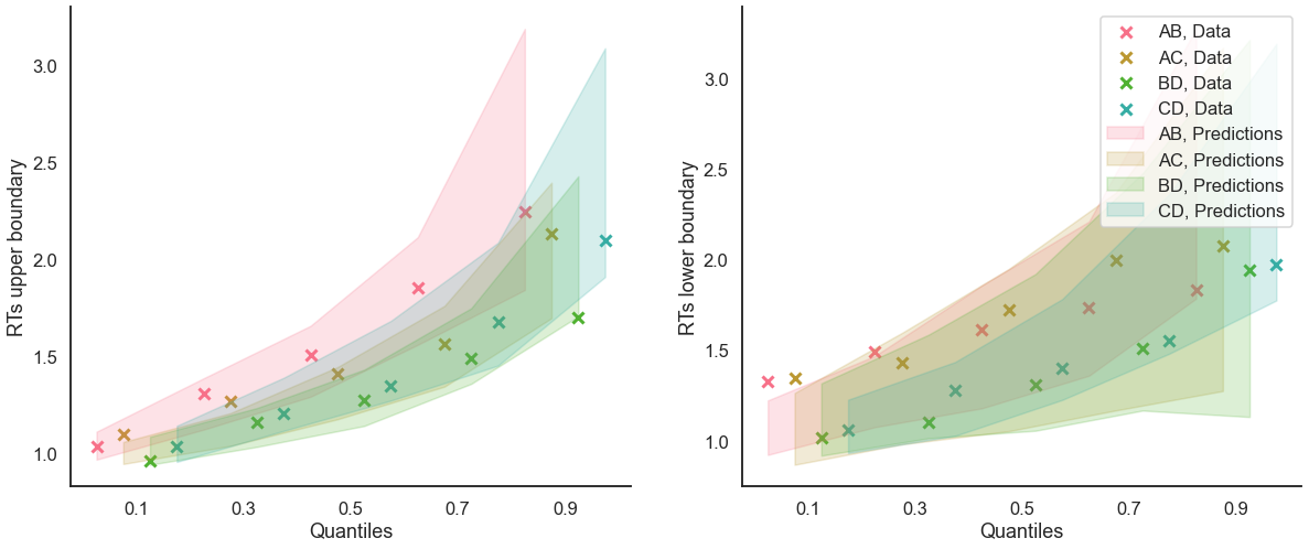
../_images/notebooks_RLDDM_fitting_29_0.png

[21]:

model_fit.plot_quantiles_grouped_posterior_predictives(
    n_posterior_predictives=300,
    grouping_var='choice_pair',
    palette = sns.color_palette('husl'),
    intervals_kws={'alpha': .3, 'lw':8},
    hue_order=['AB', 'AC', 'BD', 'CD'],
    hue_labels=['ab', 'ac', 'bd', 'cd']);

../_images/notebooks_RLDDM_fitting_30_0.png