Fit the DDM on individual data

[1]:

import rlssm
import pandas as pd
import os

Import the data

[2]:

data = rlssm.load_example_dataset(hierarchical_levels = 1)

data.head()

[2]:

	participant	block_label	trial_block	f_cor	f_inc	cor_option	inc_option	times_seen	rt	accuracy
0	15	1	1	50	28	3	1	1	2.630658	1
1	15	1	2	52	44	3	1	2	2.718299	1
2	15	1	3	30	38	2	1	2	2.382882	1
3	15	1	4	64	45	4	2	1	2.167205	1
4	15	1	5	48	26	3	1	3	2.748257	0

Initialize the model

[3]:

model = rlssm.DDModel(hierarchical_levels = 1)

Using cached StanModel

Fit

[4]:

# sampling parameters
n_iter = 1000
n_chains = 2
n_thin = 1

[5]:

model_fit = model.fit(
    data,
    thin = n_thin,
    iter = n_iter,
    chains = n_chains,
    pointwise_waic=False,
    verbose = False)

Fitting the model using the priors:
drift_priors {'mu': 1, 'sd': 5}
threshold_priors {'mu': 0, 'sd': 5}
ndt_priors {'mu': 0, 'sd': 5}

WARNING:pystan:Maximum (flat) parameter count (1000) exceeded: skipping diagnostic tests for n_eff and Rhat.
To run all diagnostics call pystan.check_hmc_diagnostics(fit)

Checks MCMC diagnostics:
n_eff / iter looks reasonable for all parameters
0.0 of 1000 iterations ended with a divergence (0.0%)
0 of 1000 iterations saturated the maximum tree depth of 10 (0.0%)
E-BFMI indicated no pathological behavior

get Rhat

[6]:

model_fit.rhat

[6]:

	rhat	variable
0	1.000810	drift
1	1.006943	threshold
2	1.007549	ndt

get wAIC

[7]:

model_fit.waic

[7]:

{'lppd': -249.31901167684737,
 'p_waic': 3.0587189056624244,
 'waic': 504.7554611650196,
 'waic_se': 34.26010966730786}

Posteriors

[8]:

model_fit.samples.describe()

[8]:

	chain	draw	transf_drift	transf_threshold	transf_ndt
count	1000.00000	1000.000000	1000.000000	1000.000000	1000.000000
mean	0.50000	249.500000	0.887978	2.066264	0.936474
std	0.50025	144.409501	0.077742	0.078720	0.016016
min	0.00000	0.000000	0.639946	1.866531	0.871589
25%	0.00000	124.750000	0.838996	2.012143	0.926123
50%	0.50000	249.500000	0.887060	2.060566	0.938202
75%	1.00000	374.250000	0.939397	2.117163	0.948530
max	1.00000	499.000000	1.172651	2.364307	0.971738

[9]:

import seaborn as sns
sns.set(context = "talk",
        style = "white",
        palette = "husl",
        rc={'figure.figsize':(15, 8)})

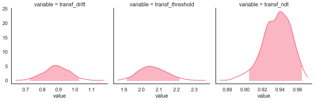
[10]:

model_fit.plot_posteriors(height=5, show_intervals="HDI", alpha_intervals=.05);

../_images/notebooks_DDM_fitting_16_0.png

Posterior predictives

Ungrouped

[11]:

pp = model_fit.get_posterior_predictives_df(n_posterior_predictives=100)
pp

[11]:

variable	rt										...	accuracy
trial	1	2	3	4	5	6	7	8	9	10	...	230	231	232	233	234	235	236	237	238	239
sample
1	1.223334	2.259334	1.509334	1.212334	2.187334	2.319334	1.228334	2.348334	1.991334	1.349334	...	1.0	1.0	1.0	0.0	1.0	1.0	0.0	1.0	1.0	0.0
2	1.305570	1.567570	1.483570	1.874570	1.748570	1.159570	1.312570	1.802570	1.703570	1.095570	...	1.0	1.0	1.0	1.0	1.0	1.0	1.0	1.0	1.0	1.0
3	1.400020	1.402020	3.388020	1.057020	2.142020	1.223020	2.474020	1.597020	1.396020	1.279020	...	1.0	1.0	1.0	1.0	1.0	1.0	0.0	1.0	0.0	1.0
4	4.672817	1.878817	1.780817	1.547817	2.339817	1.494817	1.835817	1.222817	2.578817	3.279817	...	0.0	1.0	1.0	1.0	1.0	1.0	1.0	1.0	1.0	1.0
5	3.312260	2.279260	2.675260	1.332260	1.425260	2.339260	1.814260	1.268260	1.372260	1.549260	...	0.0	1.0	0.0	1.0	1.0	1.0	1.0	1.0	1.0	1.0
...	...	...	...	...	...	...	...	...	...	...	...	...	...	...	...	...	...	...	...	...	...
96	2.024093	1.262093	2.446093	4.031093	1.437093	1.193093	2.746093	1.450093	1.216093	2.919093	...	1.0	1.0	1.0	1.0	0.0	1.0	1.0	0.0	0.0	1.0
97	1.300279	1.493279	1.214279	1.889279	1.611279	1.160279	1.265279	1.881279	3.004279	2.891279	...	1.0	1.0	0.0	1.0	1.0	0.0	1.0	1.0	1.0	1.0
98	1.342920	1.468920	2.064920	1.563920	3.481920	1.511920	1.863920	1.289920	1.685920	1.471920	...	1.0	1.0	1.0	1.0	1.0	1.0	1.0	1.0	0.0	1.0
99	1.473277	2.308277	1.750277	1.995277	1.345277	1.712277	1.291277	1.392277	1.486277	1.976277	...	1.0	1.0	1.0	1.0	1.0	0.0	1.0	1.0	1.0	1.0
100	1.485624	1.479624	1.893624	2.016624	1.354624	2.434624	1.665624	2.441624	1.143624	1.129624	...	1.0	1.0	0.0	1.0	1.0	1.0	1.0	1.0	1.0	1.0

100 rows × 478 columns

[12]:

pp_summary = model_fit.get_posterior_predictives_summary(n_posterior_predictives=100)
pp_summary

[12]:

	mean_accuracy	mean_rt	skewness	quant_10_rt_low	quant_30_rt_low	quant_50_rt_low	quant_70_rt_low	quant_90_rt_low	quant_10_rt_up	quant_30_rt_up	quant_50_rt_up	quant_70_rt_up	quant_90_rt_up
sample
1	0.878661	1.892451	2.078444	1.378734	1.538534	1.742334	2.037534	3.194934	1.212934	1.432634	1.656334	2.048934	2.963734
2	0.832636	1.769654	3.328429	1.184570	1.293470	1.441070	1.742370	2.202970	1.185370	1.381770	1.575570	1.923370	2.626970
3	0.924686	1.782321	1.752938	1.219020	1.453120	1.737520	1.887220	2.282020	1.230020	1.360020	1.584020	1.929020	2.615020
4	0.803347	1.767152	1.387015	1.225617	1.505617	1.725817	1.867217	2.265217	1.175917	1.353117	1.589317	1.994917	2.578117
5	0.895397	1.745301	2.373022	1.250060	1.413660	1.624260	1.853460	2.186860	1.179860	1.352760	1.582260	1.840360	2.588060
...	...	...	...	...	...	...	...	...	...	...	...	...	...
96	0.849372	1.825122	2.236298	1.277593	1.400593	1.548593	1.712593	2.730093	1.198093	1.389893	1.613093	2.038493	2.657093
97	0.874477	1.747479	1.793196	1.177179	1.235679	1.505779	1.718079	2.450379	1.171479	1.301479	1.504279	1.795079	2.846879
98	0.836820	1.865740	1.573733	1.221320	1.324320	1.529920	1.825520	2.247520	1.200220	1.433020	1.740920	2.032520	2.920520
99	0.887029	1.832696	1.897374	1.208077	1.358877	1.609277	1.928877	2.915877	1.184377	1.371877	1.601277	2.000277	2.812677
100	0.870293	1.697068	2.067900	1.206624	1.279624	1.573624	1.868624	2.586624	1.143124	1.328724	1.525124	1.824924	2.440624

100 rows × 13 columns

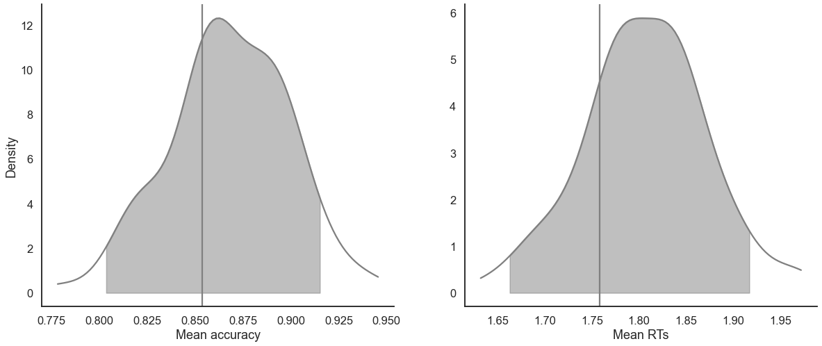
[13]:

model_fit.plot_mean_posterior_predictives(n_posterior_predictives=100, figsize=(20,8), show_intervals='HDI');

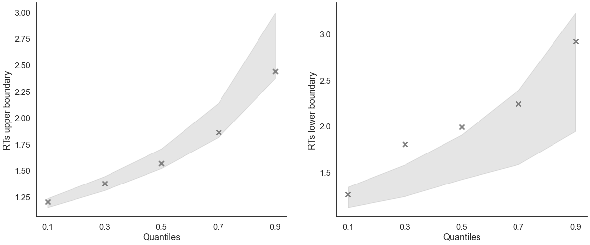
../_images/notebooks_DDM_fitting_21_0.png

[14]:

model_fit.plot_quantiles_posterior_predictives(n_posterior_predictives=100, kind='shades');

../_images/notebooks_DDM_fitting_22_0.png

Grouped

[15]:

import numpy as np

[16]:

# Define new grouping variables, in this case, for the different choice pairs, but any grouping var can do
data['choice_pair'] = 'AB'
data.loc[(data.cor_option == 3) & (data.inc_option == 1), 'choice_pair'] = 'AC'
data.loc[(data.cor_option == 4) & (data.inc_option == 2), 'choice_pair'] = 'BD'
data.loc[(data.cor_option == 4) & (data.inc_option == 3), 'choice_pair'] = 'CD'

data['block_bins'] = pd.cut(data.trial_block, 8, labels=np.arange(1, 9))

[17]:

model_fit.get_grouped_posterior_predictives_summary(
                grouping_vars=['block_label', 'choice_pair'],
                quantiles=[.3, .5, .7],
                n_posterior_predictives=100)

[17]:

			mean_accuracy	mean_rt	skewness	quant_30_rt_low	quant_30_rt_up	quant_50_rt_low	quant_50_rt_up	quant_70_rt_low	quant_70_rt_up
block_label	choice_pair	sample
1	AB	1	0.85	2.110784	1.247609	1.394134	1.324534	1.427334	1.898334	1.492934	2.750934
		2	0.85	1.624170	0.995058	1.831370	1.357170	2.268570	1.439570	2.271770	1.612570
		3	0.95	1.735570	1.643538	1.350020	1.374820	1.350020	1.546020	1.350020	1.817820
		4	0.75	1.557317	1.365500	1.221417	1.320417	1.239817	1.503817	1.509417	1.694217
		5	0.85	1.756110	1.313400	1.313460	1.244660	1.338260	1.565260	1.588660	2.090260
...	...	...	...	...	...	...	...	...	...	...	...
3	CD	96	0.75	1.501643	0.760884	1.369893	1.277693	1.553093	1.382093	1.657093	1.625293
		97	1.00	1.679479	1.992939	NaN	1.343079	NaN	1.527279	NaN	1.597579
		98	1.00	1.809320	2.061042	NaN	1.290220	NaN	1.469920	NaN	1.932820
		99	0.95	1.526577	1.452011	1.913277	1.293877	1.913277	1.353277	1.913277	1.658677
		100	0.85	1.690874	2.286446	1.749624	1.329624	1.943624	1.404624	1.964424	1.777024

1200 rows × 9 columns

[18]:

model_fit.get_grouped_posterior_predictives_summary(
                grouping_vars=['block_bins'],
                quantiles=[.3, .5, .7],
                n_posterior_predictives=100)

[18]:

		mean_accuracy	mean_rt	skewness	quant_30_rt_low	quant_30_rt_up	quant_50_rt_low	quant_50_rt_up	quant_70_rt_low	quant_70_rt_up
block_bins	sample
1	1	0.933333	1.963768	1.036143	1.866334	1.523834	2.112334	1.723834	2.358334	2.232334
	2	0.833333	1.588937	2.913381	1.240770	1.281170	1.549570	1.446570	1.569570	1.629170
	3	0.933333	1.896486	2.235551	1.538420	1.590420	1.672020	1.839520	1.805620	2.031920
	4	0.833333	1.723484	1.037996	1.675017	1.328017	1.723817	1.482817	1.995017	1.927617
	5	0.966667	1.668193	2.396271	2.047260	1.285660	2.047260	1.446260	2.047260	1.650460
...	...	...	...	...	...	...	...	...	...	...
8	96	0.689655	1.988265	1.413794	1.474693	1.529093	1.514093	1.859093	2.040893	2.171193
	97	0.793103	1.831796	1.107177	1.467779	1.469279	1.586779	1.549279	1.791779	2.077879
	98	0.793103	1.898368	2.873183	1.320920	1.476520	1.478920	1.701920	1.585420	2.138520
	99	0.896552	2.043208	2.130396	1.331477	1.459777	1.346277	1.714277	1.890677	2.075277
	100	0.965517	1.748003	1.149147	1.250624	1.506824	1.250624	1.692624	1.250624	1.907424

800 rows × 9 columns

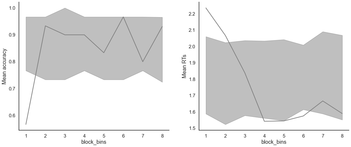
[19]:

model_fit.plot_mean_grouped_posterior_predictives(grouping_vars=['block_bins'],
                                                  n_posterior_predictives=100,
                                                  figsize=(20,8));

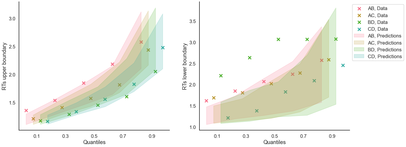
../_images/notebooks_DDM_fitting_28_0.png

[20]:

model_fit.plot_quantiles_grouped_posterior_predictives(
    n_posterior_predictives=100,
    grouping_var='choice_pair',
    kind='shades',
    quantiles=[.1, .3, .5, .7, .9]);

../_images/notebooks_DDM_fitting_29_0.png