Parameter recovery of the hierarchical DDM with starting point bias

import rlssm
import pandas as pd

Simulate group data

from rlssm.random import simulate_hier_ddm

data = simulate_hier_ddm(n_trials=200,
                         n_participants=10,
                         gen_mu_drift=.6, gen_sd_drift=.1,
                         gen_mu_threshold=.5, gen_sd_threshold=.1,
                         gen_mu_ndt=0, gen_sd_ndt=.01,
                         gen_mu_rel_sp=.1, gen_sd_rel_sp=.01)

data.head()

		drift	threshold	ndt	rel_sp	rt	accuracy
participant	trial
1	1	0.623365	0.997041	0.692471	0.539151	0.716471	1.0
	1	0.623365	0.997041	0.692471	0.539151	0.902471	1.0
	1	0.623365	0.997041	0.692471	0.539151	0.793471	1.0
	1	0.623365	0.997041	0.692471	0.539151	0.980471	0.0
	1	0.623365	0.997041	0.692471	0.539151	1.739471	1.0

data.groupby('participant').describe()[['rt', 'accuracy']]

	rt								accuracy
	count	mean	std	min	25%	50%	75%	max	count	mean	std	min	25%	50%	75%	max
participant
1	200.0	0.951961	0.228372	0.710471	0.796221	0.888471	1.012721	2.130471	200.0	0.680	0.467647	0.0	0.0	1.0	1.0	1.0
2	200.0	0.977915	0.226304	0.730590	0.816340	0.919590	1.074590	2.046590	200.0	0.650	0.478167	0.0	0.0	1.0	1.0	1.0
3	200.0	0.999711	0.246408	0.728586	0.829836	0.935586	1.111336	2.373586	200.0	0.675	0.469550	0.0	0.0	1.0	1.0	1.0
4	200.0	0.926358	0.171244	0.720133	0.794883	0.892133	1.008383	1.610133	200.0	0.695	0.461563	0.0	0.0	1.0	1.0	1.0
5	200.0	0.885120	0.165347	0.708605	0.774355	0.831605	0.923105	1.585605	200.0	0.625	0.485338	0.0	0.0	1.0	1.0	1.0
6	200.0	0.939961	0.198498	0.711296	0.809296	0.900296	1.028546	2.424296	200.0	0.655	0.476561	0.0	0.0	1.0	1.0	1.0
7	200.0	0.909842	0.185368	0.703557	0.785057	0.844057	0.984807	2.023557	200.0	0.720	0.450126	0.0	0.0	1.0	1.0	1.0
8	200.0	0.902757	0.165986	0.710047	0.790047	0.854547	0.967047	1.645047	200.0	0.635	0.482638	0.0	0.0	1.0	1.0	1.0
9	200.0	0.892931	0.151139	0.711606	0.777356	0.852106	0.968856	1.604606	200.0	0.735	0.442441	0.0	0.0	1.0	1.0	1.0
10	200.0	0.955701	0.230286	0.726306	0.810306	0.901306	1.023556	2.345306	200.0	0.705	0.457187	0.0	0.0	1.0	1.0	1.0

Initialize the model

model = rlssm.DDModel(hierarchical_levels = 2, starting_point_bias=True)

Using cached StanModel

Fit

# sampling parameters
n_iter = 5000
n_chains = 2
n_thin = 1

model_fit = model.fit(
    data,
    thin = n_thin,
    iter = n_iter,
    chains = n_chains,
    verbose = False)

Fitting the model using the priors:
drift_priors {'mu_mu': 1, 'sd_mu': 5, 'mu_sd': 0, 'sd_sd': 5}
threshold_priors {'mu_mu': 1, 'sd_mu': 3, 'mu_sd': 0, 'sd_sd': 3}
ndt_priors {'mu_mu': 1, 'sd_mu': 1, 'mu_sd': 0, 'sd_sd': 1}
rel_sp_priors {'mu_mu': 0, 'sd_mu': 1, 'mu_sd': 0, 'sd_sd': 1}

WARNING:pystan:Maximum (flat) parameter count (1000) exceeded: skipping diagnostic tests for n_eff and Rhat.
To run all diagnostics call pystan.check_hmc_diagnostics(fit)
WARNING:pystan:3 of 5000 iterations ended with a divergence (0.06 %).
WARNING:pystan:Try running with adapt_delta larger than 0.8 to remove the divergences.

Checks MCMC diagnostics:
n_eff / iter looks reasonable for all parameters
3.0 of 5000 iterations ended with a divergence (0.06%)
  Try running with larger adapt_delta to remove the divergences
0 of 5000 iterations saturated the maximum tree depth of 10 (0.0%)
E-BFMI indicated no pathological behavior

get Rhat

model_fit.rhat.describe()

	rhat
count	48.000000
mean	1.000329
std	0.000791
min	0.999604
25%	0.999880
50%	1.000038
75%	1.000444
max	1.003618

calculate wAIC

model_fit.waic

{'lppd': -138.87336841598818,
 'p_waic': 23.687615971055777,
 'waic': 325.1219687740879,
 'waic_se': 92.20297977041197}

Posteriors

model_fit.samples.describe()

	chain	draw	transf_mu_drift	transf_mu_threshold	transf_mu_ndt	transf_mu_rel_sp	drift_sbj[1]	drift_sbj[2]	drift_sbj[3]	drift_sbj[4]	...	rel_sp_sbj[1]	rel_sp_sbj[2]	rel_sp_sbj[3]	rel_sp_sbj[4]	rel_sp_sbj[5]	rel_sp_sbj[6]	rel_sp_sbj[7]	rel_sp_sbj[8]	rel_sp_sbj[9]	rel_sp_sbj[10]
count	5000.00000	5000.000000	5000.000000	5000.000000	5000.000000	5000.000000	5000.000000	5000.000000	5000.000000	5000.000000	...	5000.000000	5000.000000	5000.000000	5000.000000	5000.000000	5000.000000	5000.000000	5000.000000	5000.000000	5000.000000
mean	0.50000	1249.500000	0.615952	1.009498	0.691726	0.530285	0.603799	0.576879	0.599734	0.642007	...	0.536195	0.526231	0.522930	0.526576	0.520650	0.492087	0.568101	0.520123	0.549857	0.539313
std	0.50005	721.759958	0.065815	0.030910	0.002199	0.012904	0.090243	0.093931	0.088017	0.093087	...	0.018094	0.017883	0.018320	0.017435	0.017763	0.020995	0.021740	0.017393	0.019104	0.018017
min	0.00000	0.000000	0.350688	0.860374	0.681198	0.475725	0.093595	0.157550	0.190691	0.282644	...	0.469905	0.460770	0.455520	0.465381	0.450294	0.414656	0.506434	0.461902	0.484085	0.466391
25%	0.00000	624.750000	0.572878	0.990568	0.690373	0.522065	0.549763	0.520853	0.544895	0.581498	...	0.524433	0.514626	0.510905	0.515375	0.509454	0.477564	0.552796	0.508784	0.536325	0.527094
50%	0.50000	1249.500000	0.615384	1.009284	0.691617	0.530185	0.604913	0.584693	0.601593	0.633981	...	0.535846	0.526326	0.523374	0.527026	0.521320	0.492551	0.567758	0.520566	0.549263	0.538623
75%	1.00000	1874.250000	0.659705	1.028144	0.693001	0.538358	0.660774	0.638983	0.656278	0.694858	...	0.548069	0.537657	0.535127	0.538225	0.532493	0.506852	0.582966	0.531734	0.562528	0.551173
max	1.00000	2499.000000	0.961835	1.160558	0.704329	0.589211	0.934712	0.990759	0.994084	1.178273	...	0.602393	0.590122	0.599665	0.592212	0.595451	0.551932	0.638467	0.586136	0.617997	0.610974

8 rows × 46 columns

import seaborn as sns
sns.set(context = "talk",
        style = "white",
        palette = "husl",
        rc={'figure.figsize':(15, 8)})

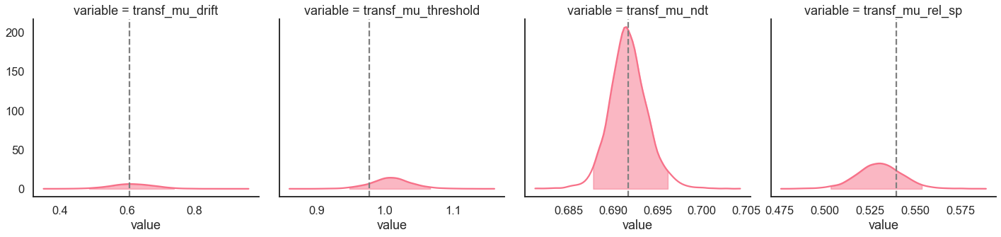
Here we plot the estimated posterior distributions against the generating parameters, to see whether the model parameters are recovering well:

g = model_fit.plot_posteriors(height=5, show_intervals='HDI')

for i, ax in enumerate(g.axes.flatten()):
    ax.axvline(data[['drift', 'threshold', 'ndt', 'rel_sp']].mean().values[i], color='grey', linestyle='--')