Fit the DDM on hierarchical data

[1]:

import rlssm
import pandas as pd
import os

Import the data

[2]:

data = rlssm.load_example_dataset(hierarchical_levels = 2)

data.head()

[2]:

	participant	block_label	trial_block	f_cor	f_inc	cor_option	inc_option	times_seen	rt	accuracy
0	1	1	1	43	39	2	1	1	1.244082	0
1	1	1	2	60	50	4	3	1	1.101821	1
2	1	1	3	44	36	4	2	2	1.029923	0
3	1	1	4	55	55	4	3	2	1.368007	0
4	1	1	5	52	49	4	3	3	1.039329	1

Initialize the model

[3]:

model = rlssm.DDModel(hierarchical_levels = 2)

Using cached StanModel

Fit

[4]:

# sampling parameters
n_iter = 3000
n_warmup = 1000
n_chains = 2
n_thin = 1

# bayesian model, change default priors:
drift_priors = {'mu_mu':1, 'sd_mu':1, 'mu_sd':0, 'sd_sd':1}
threshold_priors = {'mu_mu':-1, 'sd_mu':.5, 'mu_sd':0, 'sd_sd':1}

[5]:

model_fit = model.fit(
    data,
    drift_priors=drift_priors,
    threshold_priors=threshold_priors,
    warmup = n_warmup,
    iter = n_iter,
    chains = n_chains,
    verbose = False)

Fitting the model using the priors:
drift_priors {'mu_mu': 1, 'sd_mu': 1, 'mu_sd': 0, 'sd_sd': 1}
threshold_priors {'mu_mu': -1, 'sd_mu': 0.5, 'mu_sd': 0, 'sd_sd': 1}
ndt_priors {'mu_mu': 1, 'sd_mu': 1, 'mu_sd': 0, 'sd_sd': 1}

WARNING:pystan:Maximum (flat) parameter count (1000) exceeded: skipping diagnostic tests for n_eff and Rhat.
To run all diagnostics call pystan.check_hmc_diagnostics(fit)

Checks MCMC diagnostics:
n_eff / iter looks reasonable for all parameters
0.0 of 4000 iterations ended with a divergence (0.0%)
0 of 4000 iterations saturated the maximum tree depth of 10 (0.0%)
E-BFMI indicated no pathological behavior

get Rhat

[6]:

model_fit.rhat.describe()

[6]:

	rhat
count	87.000000
mean	1.002063
std	0.001658
min	0.999537
25%	1.000544
50%	1.001811
75%	1.003711
max	1.005368

calculate wAIC

[7]:

model_fit.waic

[7]:

{'lppd': -5411.232334273516,
 'p_waic': 100.49218768903286,
 'waic': 11023.449043925099,
 'waic_se': 176.56475211992282}

Posteriors

[8]:

model_fit.samples.describe()

[8]:

	chain	draw	transf_mu_drift	transf_mu_threshold	transf_mu_ndt	drift_sbj[1]	drift_sbj[2]	drift_sbj[3]	drift_sbj[4]	drift_sbj[5]	...	ndt_sbj[18]	ndt_sbj[19]	ndt_sbj[20]	ndt_sbj[21]	ndt_sbj[22]	ndt_sbj[23]	ndt_sbj[24]	ndt_sbj[25]	ndt_sbj[26]	ndt_sbj[27]
count	4000.000000	4000.000000	4000.000000	4000.000000	4000.000000	4000.000000	4000.000000	4000.000000	4000.000000	4000.000000	...	4000.000000	4000.000000	4000.000000	4000.000000	4000.000000	4000.000000	4000.000000	4000.000000	4000.000000	4000.000000
mean	0.500000	999.500000	0.902761	1.807539	0.741604	1.130521	0.796869	0.987316	0.722244	0.788625	...	0.730397	0.387217	0.917420	0.746415	0.742279	0.582877	0.738693	0.853545	0.465463	0.863420
std	0.500063	577.422379	0.059822	0.054908	0.026017	0.092552	0.086190	0.091410	0.070307	0.080458	...	0.010526	0.013373	0.012058	0.016956	0.012844	0.015244	0.011544	0.009388	0.005858	0.013867
min	0.000000	0.000000	0.674924	1.595346	0.647802	0.819075	0.466966	0.655683	0.454312	0.505320	...	0.676340	0.326232	0.861828	0.663290	0.685504	0.512557	0.690101	0.785180	0.433751	0.801070
25%	0.000000	499.750000	0.863994	1.772357	0.723955	1.067871	0.738409	0.926912	0.674731	0.733996	...	0.723725	0.378700	0.909887	0.735585	0.734626	0.573140	0.731390	0.847871	0.461699	0.854582
50%	0.500000	999.500000	0.903058	1.808784	0.740936	1.130679	0.795897	0.986899	0.722107	0.788834	...	0.731266	0.388043	0.918484	0.747791	0.743200	0.583825	0.739453	0.854248	0.465894	0.864309
75%	1.000000	1499.250000	0.940805	1.842290	0.758722	1.192259	0.855532	1.047859	0.769020	0.842797	...	0.738054	0.396858	0.925692	0.758399	0.751337	0.593646	0.746683	0.860238	0.469833	0.873388
max	1.000000	1999.000000	1.141893	2.033432	0.852444	1.422928	1.123298	1.392205	0.987737	1.074931	...	0.757969	0.422315	0.950412	0.794461	0.777875	0.625252	0.774845	0.880258	0.479346	0.901650

8 rows × 86 columns

[9]:

import seaborn as sns
sns.set(context = "talk",
        style = "white",
        palette = "husl",
        rc={'figure.figsize':(15, 8)})

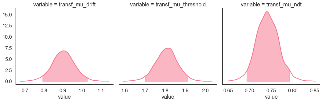
[10]:

model_fit.plot_posteriors(height=5, show_intervals='HDI');

../_images/notebooks_DDM_hierarchical_fitting_16_0.png

Posterior predictives

Ungrouped

[11]:

pp_summary = model_fit.get_posterior_predictives_summary(n_posterior_predictives=100)
pp_summary

[11]:

	mean_accuracy	mean_rt	skewness	quant_10_rt_low	quant_30_rt_low	quant_50_rt_low	quant_70_rt_low	quant_90_rt_low	quant_10_rt_up	quant_30_rt_up	quant_50_rt_up	quant_70_rt_up	quant_90_rt_up
sample
1	0.833075	1.465869	1.924414	0.883730	1.093301	1.272597	1.568961	2.198967	0.941062	1.119104	1.321842	1.611800	2.195939
2	0.836170	1.463162	2.103788	0.892418	1.078721	1.299354	1.572111	2.172324	0.931466	1.112196	1.298555	1.591849	2.215945
3	0.846999	1.483644	2.208010	0.905064	1.090908	1.315067	1.576960	2.248927	0.940345	1.116395	1.311158	1.604061	2.271693
4	0.814047	1.484810	2.045138	0.923073	1.095670	1.295465	1.581610	2.274091	0.947493	1.129157	1.314156	1.610896	2.241961
5	0.837407	1.465835	2.270638	0.922109	1.093109	1.314665	1.643438	2.282154	0.937676	1.112792	1.289724	1.571149	2.203733
...	...	...	...	...	...	...	...	...	...	...	...	...	...
96	0.829517	1.469527	2.031207	0.921734	1.093067	1.290120	1.542060	2.201835	0.940105	1.114216	1.305271	1.599589	2.227620
97	0.834004	1.482221	2.272835	0.884389	1.096907	1.286055	1.565813	2.301758	0.940277	1.119118	1.309424	1.595480	2.277529
98	0.825959	1.478508	2.217464	0.900590	1.089122	1.268247	1.549817	2.153399	0.941824	1.118637	1.309469	1.600631	2.277239
99	0.828899	1.468675	2.238373	0.900192	1.104152	1.303109	1.600759	2.304936	0.932834	1.107752	1.296001	1.570841	2.213527
100	0.827042	1.463481	2.305245	0.882360	1.074106	1.280296	1.583718	2.223310	0.945467	1.117998	1.303640	1.580593	2.195555

100 rows × 13 columns

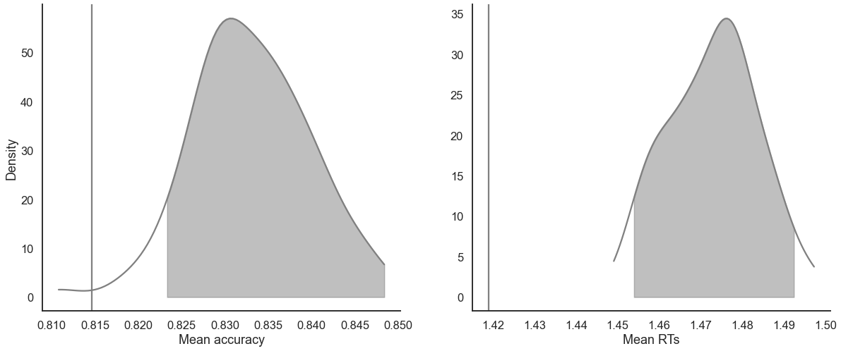
[12]:

model_fit.plot_mean_posterior_predictives(n_posterior_predictives=100, figsize=(20,8), show_intervals='HDI');

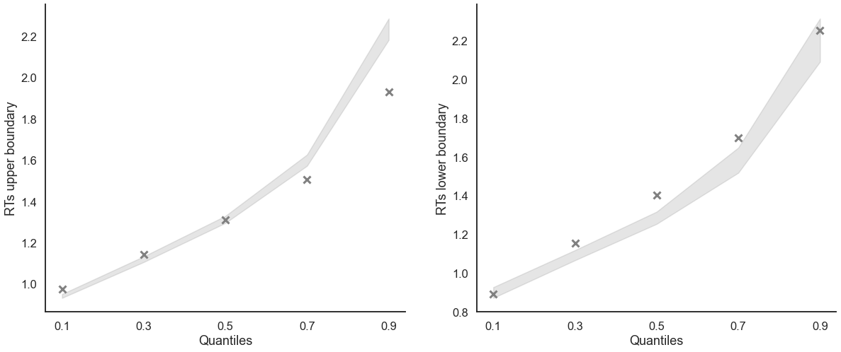
../_images/notebooks_DDM_hierarchical_fitting_20_0.png

[13]:

model_fit.plot_quantiles_posterior_predictives(n_posterior_predictives=100, kind='shades');

../_images/notebooks_DDM_hierarchical_fitting_21_0.png

Grouped

[14]:

import numpy as np

[15]:

# Define new grouping variables, in this case, for the different choice pairs, but any grouping var can do
data['choice_pair'] = 'AB'
data.loc[(data.cor_option == 3) & (data.inc_option == 1), 'choice_pair'] = 'AC'
data.loc[(data.cor_option == 4) & (data.inc_option == 2), 'choice_pair'] = 'BD'
data.loc[(data.cor_option == 4) & (data.inc_option == 3), 'choice_pair'] = 'CD'

data['block_bins'] = pd.cut(data.trial_block, 8, labels=np.arange(1, 9))

[16]:

model_fit.get_grouped_posterior_predictives_summary(
                grouping_vars=['block_label', 'choice_pair'],
                quantiles=[.3, .5, .7],
                n_posterior_predictives=100)

[16]:

			mean_accuracy	mean_rt	skewness	quant_30_rt_low	quant_30_rt_up	quant_50_rt_low	quant_50_rt_up	quant_70_rt_low	quant_70_rt_up
block_label	choice_pair	sample
1	AB	1	0.836127	1.424913	1.829896	1.132202	1.090361	1.302380	1.287831	1.640282	1.555307
		2	0.810056	1.489926	3.021606	1.085730	1.115178	1.290275	1.313489	1.660278	1.574471
		3	0.834264	1.522572	1.795817	1.114961	1.123546	1.348158	1.338346	1.773007	1.607617
		4	0.826816	1.504265	2.000594	1.127252	1.137665	1.289395	1.347707	1.620425	1.639692
		5	0.856611	1.455028	2.136628	1.016709	1.092805	1.266724	1.297497	1.535460	1.598402
...	...	...	...	...	...	...	...	...	...	...	...
3	CD	96	0.822222	1.508209	1.729570	1.070761	1.113506	1.194467	1.393401	1.542280	1.692783
		97	0.829630	1.469977	1.739914	1.114338	1.112565	1.333333	1.292743	1.630972	1.608350
		98	0.838889	1.519894	1.752790	1.191110	1.155950	1.393306	1.349036	1.715621	1.666124
		99	0.844444	1.462611	1.526917	1.011587	1.141000	1.217973	1.333668	1.496050	1.607953
		100	0.838889	1.442204	2.094030	1.070715	1.115111	1.201510	1.322007	1.432134	1.583041

1200 rows × 9 columns

[ ]:

model_fit.get_grouped_posterior_predictives_summary(
                grouping_vars=['block_bins'],
                quantiles=[.3, .5, .7],
                n_posterior_predictives=100)

[ ]:

model_fit.plot_mean_grouped_posterior_predictives(grouping_vars=['block_bins'],
                                                  n_posterior_predictives=100,
                                                  figsize=(20,8));

[ ]:

model_fit.plot_quantiles_grouped_posterior_predictives(n_posterior_predictives=100,
                                                        grouping_var='choice_pair',
                                                        kind='shades',
                                                        quantiles=[.1, .3, .5, .7, .9]);